Learning Based Image Synthesis (16-726)
Assignment 3
Aviral Agrawal (avirala)
1. Overview
This assignment revolves around training GANs and CycleGANs. Furthermore, we also dabble around with loss variations and discriminator variations. In addition, we also explore random latent space walking, spectral-normlization for increased stability in GAN training and also use an off-the shelf pre-trained Diffusion model to generate some more grumpy cats!
2. Data Augmentation
We use the following data augmentation for the 'deluxe' case :
                from torchvision.transforms import v2
                train_transform = v2.Compose([
                                v2.RandomResizedCrop(opts.image_size, antialias=True),
                                v2.RandomHorizontalFlip(),
                                v2.RandomAutocontrast(),
                                v2.ToTensor(),
                                v2.Normalize((0.5, 0.5, 0.5), (0.5, 0.5, 0.5)),
                                ])
The 'deluxe' data augmentation adds more diversity to the dataset and leads to better outputs from the model.
2. Convolution Kernel and Padding size
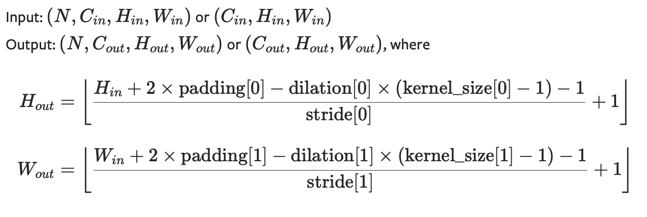
Fig1. Formula for conv2d output spatial dimension calculation
Based on the above formula, we compute the kernel size and padding size for each of the layers in the generator and discriminator as follows :
Discriminator layers :
            self.conv1 = conv(in_channels=3, out_channels=32, kernel_size=4,
                          stride=2, padding=1, norm=norm,
                          init_zero_weights=False, activ='relu')
            self.conv2 = conv(in_channels=32, out_channels=64, kernel_size=4,
                            stride=2, padding=1, norm=norm,
                            init_zero_weights=False, activ='relu')
            self.conv3 = conv(in_channels=64, out_channels=128, kernel_size=4,
                            stride=2, padding=1, norm=norm,
                            init_zero_weights=False, activ='relu')
            self.conv4 = conv(in_channels=128, out_channels=256, kernel_size=4,
                            stride=2, padding=1, norm=norm,
                            init_zero_weights=False, activ='relu')
            self.conv5 = conv(in_channels=256, out_channels=1, kernel_size=4,
                            stride=2, padding=0, norm=None,
                            init_zero_weights=False, activ='sigmoid')
Generator layers :
            self.up_conv1 = conv(in_channels=noise_size, out_channels=256,
                                kernel_size=4, stride=1, padding=3,
                                norm='instance', activ='relu')
            self.up_conv2 = up_conv(in_channels=256, out_channels=128,
                                    kernel_size=3, stride=1, padding=1,
                                    scale_factor=2, norm='instance', activ='relu')
            self.up_conv3 = up_conv(in_channels=128, out_channels=64,
                                    kernel_size=3, stride=1, padding=1,
                                    scale_factor=2, norm='instance', activ='relu')
            self.up_conv4 = up_conv(in_channels=64, out_channels=32,
                                    kernel_size=3, stride=1, padding=1,
                                    scale_factor=2, norm='instance', activ='relu')
            self.up_conv5 = up_conv(in_channels=32, out_channels=3,
                                    kernel_size=3, stride=1, padding=1,
                                    scale_factor=2, norm=None, activ='tanh')
3. Deep Convolutional Generative Adversarial Networks (DCGANs)
A DCGAN, or a Deep Convolutional Generative Adversarial Network, employs a convolutional neural network for the discriminator and a network comprising transposed convolutions for the generator. However, in this particular task, instead of utilizing transposed convolutions, we will employ a blend of an upsampling layer and a convolutional layer to serve as substitutes.
from torchvision.transforms import v2
train_transform = v2.Compose([
v2.RandomResizedCrop(opts.image_size, antialias=True),
v2.RandomHorizontalFlip(),
v2.RandomAutocontrast(),
v2.ToTensor(),
v2.Normalize((0.5, 0.5, 0.5), (0.5, 0.5, 0.5)),
])
The 'deluxe' data augmentation adds more diversity to the dataset and leads to better outputs from the model.
2. Convolution Kernel and Padding size

Fig1. Formula for conv2d output spatial dimension calculation
Based on the above formula, we compute the kernel size and padding size for each of the layers in the generator and discriminator as follows :
Discriminator layers :
self.conv1 = conv(in_channels=3, out_channels=32, kernel_size=4,
stride=2, padding=1, norm=norm,
init_zero_weights=False, activ='relu')
self.conv2 = conv(in_channels=32, out_channels=64, kernel_size=4,
stride=2, padding=1, norm=norm,
init_zero_weights=False, activ='relu')
self.conv3 = conv(in_channels=64, out_channels=128, kernel_size=4,
stride=2, padding=1, norm=norm,
init_zero_weights=False, activ='relu')
self.conv4 = conv(in_channels=128, out_channels=256, kernel_size=4,
stride=2, padding=1, norm=norm,
init_zero_weights=False, activ='relu')
self.conv5 = conv(in_channels=256, out_channels=1, kernel_size=4,
stride=2, padding=0, norm=None,
init_zero_weights=False, activ='sigmoid')
Generator layers :
self.up_conv1 = conv(in_channels=noise_size, out_channels=256,
kernel_size=4, stride=1, padding=3,
norm='instance', activ='relu')
self.up_conv2 = up_conv(in_channels=256, out_channels=128,
kernel_size=3, stride=1, padding=1,
scale_factor=2, norm='instance', activ='relu')
self.up_conv3 = up_conv(in_channels=128, out_channels=64,
kernel_size=3, stride=1, padding=1,
scale_factor=2, norm='instance', activ='relu')
self.up_conv4 = up_conv(in_channels=64, out_channels=32,
kernel_size=3, stride=1, padding=1,
scale_factor=2, norm='instance', activ='relu')
self.up_conv5 = up_conv(in_channels=32, out_channels=3,
kernel_size=3, stride=1, padding=1,
scale_factor=2, norm=None, activ='tanh')
3. Deep Convolutional Generative Adversarial Networks (DCGANs)
A DCGAN, or a Deep Convolutional Generative Adversarial Network, employs a convolutional neural network for the discriminator and a network comprising transposed convolutions for the generator. However, in this particular task, instead of utilizing transposed convolutions, we will employ a blend of an upsampling layer and a convolutional layer to serve as substitutes.

| Configuration | Generated Sample (6400 iterations) |
|---|---|
| Basic Data-Augmentation | 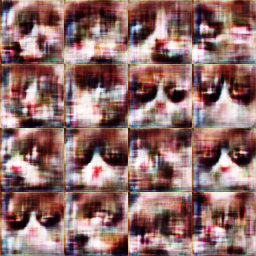 |
| Basic Data-Augmentation + Differentiable-Augmentation | 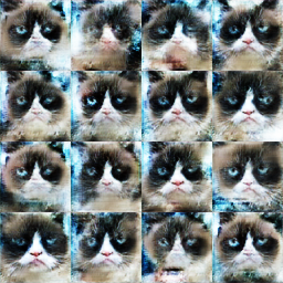 |
| Deluxe Data-Augmentation | 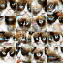 |
| Deluxe Data-Augmentation + Differentiable-Augmentation | 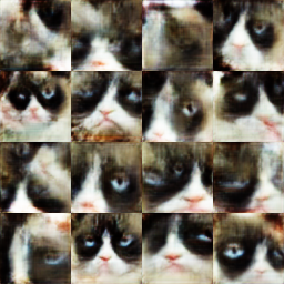 |
Following plots show the total Discriminator and Generator loss curves for the different configurations :
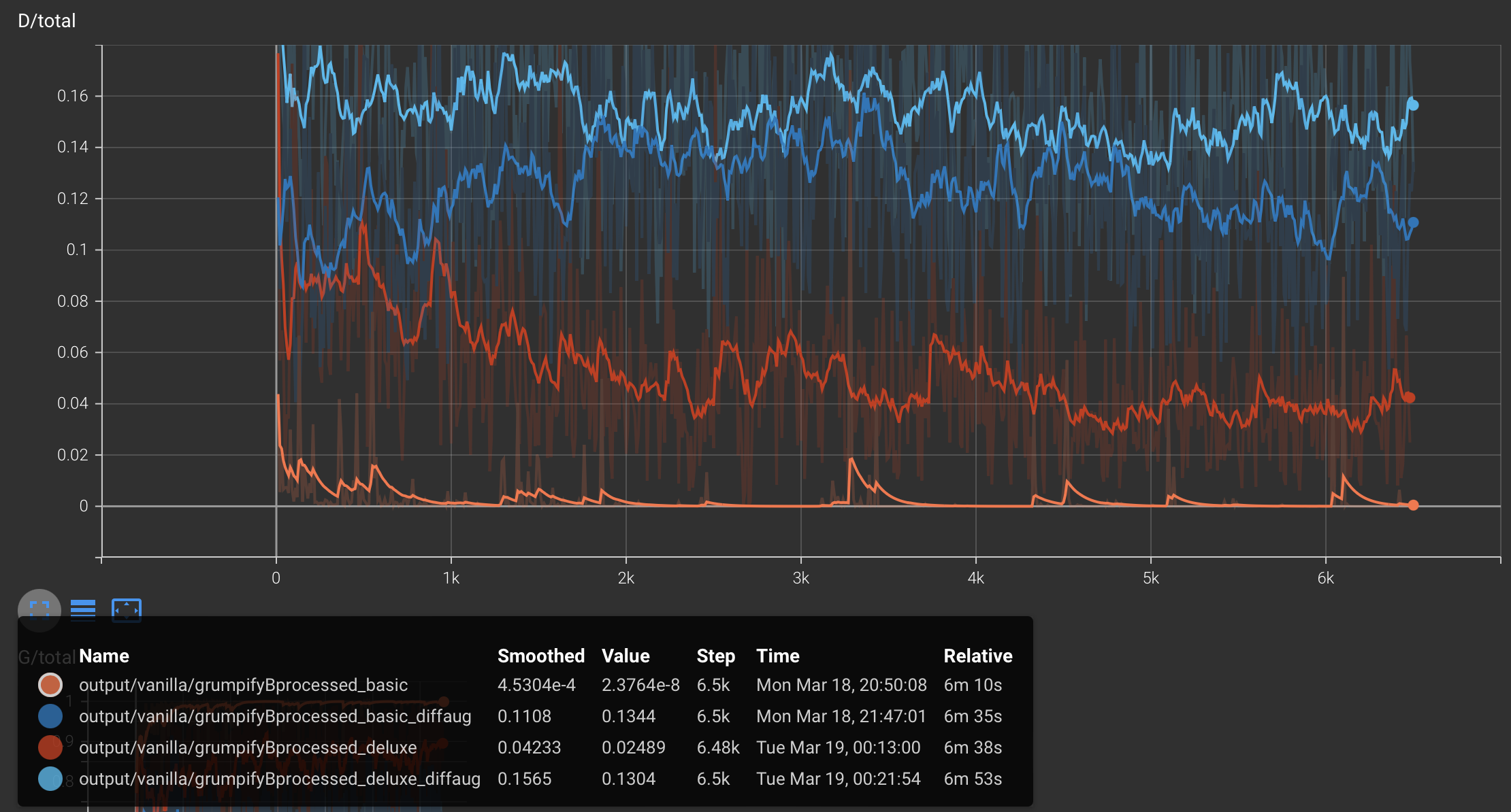
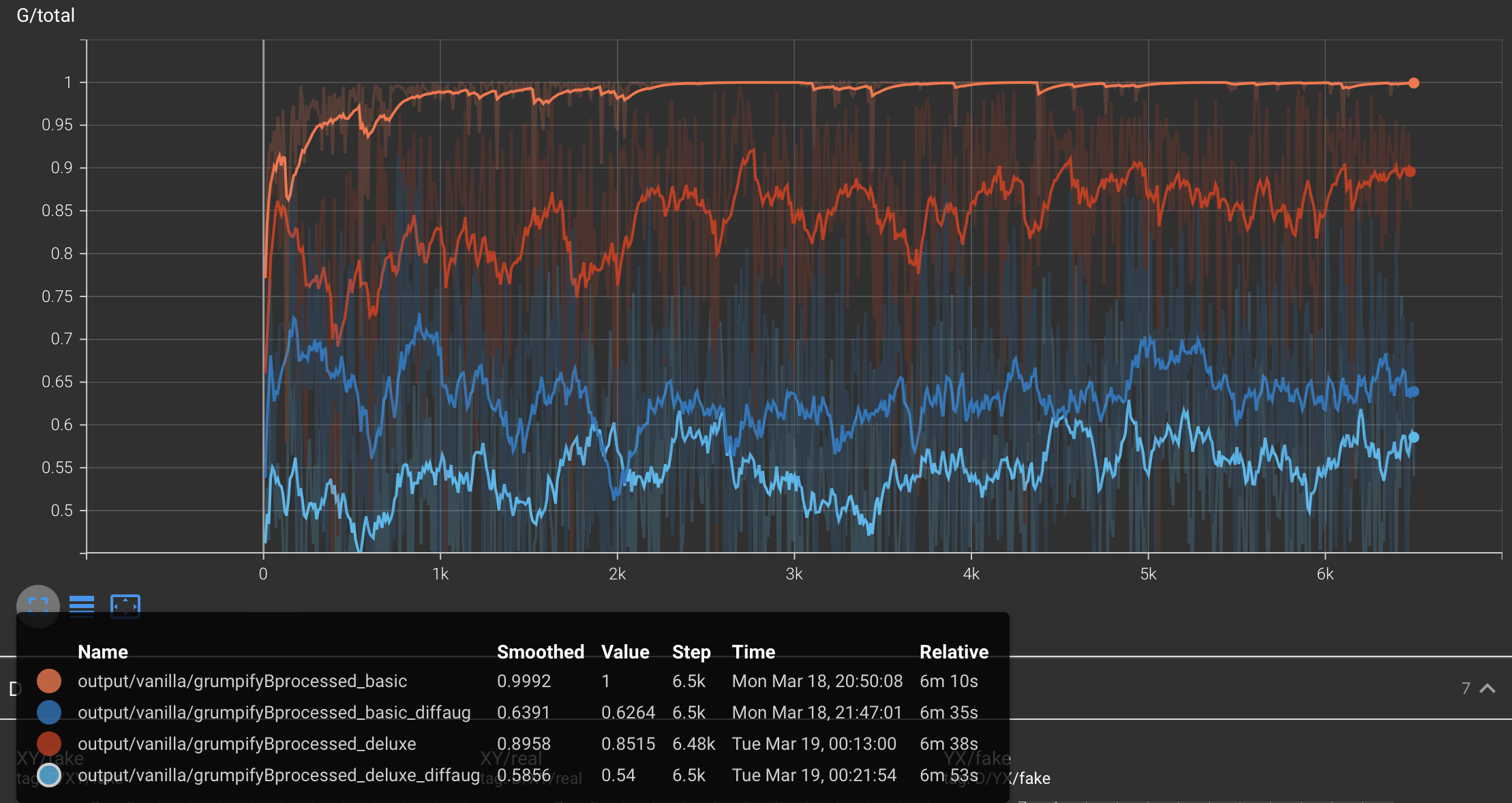
Typically, for a GAN to be 'trained', the discriminator total loss should approach 1 and the generator total loss should approach 0.5. This simply means that the discriminator cannot distinguish between real and fake images and the generator is able to generate images that are indistinguishable from real images. Hence, the discriminator gives a loss of 0.5 for both, fake and real images and the generator generates images that when fed to the discriminator, give a loss of 0.5.
Role of Data Augmentation : We see that the discriminator loss increases and the generator loss decreases (both desired behaviour) with better data augmentation, indicating that the model is learning better with better data augmentation.
Role of iterations : We see that the discriminator loss increases and the generator loss decreases (both desired behaviour) with more iterations, indicating that the model is getting better with more iterations.
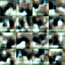

From the above samples we can see that the quality of the samples improves with more iterations (as also seen with the training curves). The samples at 6400 iterations are much better than the samples at 200 iterations. The samples at 200 iterations are more generic blobs with similar colors to cats but they lack the actual structure of a cat. The samples at 6400 iterations are much better and resemble actual cats. Hence, we can observe that the model learns broad colors easily but learning shapes takes more training.
4. CycleGAN
CycleGAN, short for Cycle-Consistent Generative Adversarial Network, consists of two generator networks and two discriminator networks, forming a cycle-consistent adversarial training scheme.
The primary objective of a CycleGAN is to learn mappings between two domains without the need for paired data. This means that it can learn to translate images from one domain to another (e.g., turning horse images into zebra images) even when there are no corresponding images between the two domains for training.
The cycle consistency loss is a key component of the CycleGAN framework. It ensures that if an image is translated from domain A to domain B and then back to domain A, it should remain close to the original image. This constraint helps in learning more accurate and realistic mappings between the domains.
| Configuration | Generated Samples (Grumpy Cats) |
|---|---|
| Disciminator = Patch, Iterations = 1000; G_XtoY | 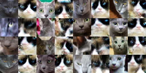 |
| Disciminator = Patch, Iterations = 1000; G_YtoX | 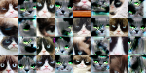 |
| Disciminator = Patch, Iterations = 1000, Cycle-consistency loss = True; G_XtoY |  |
| Disciminator = Patch, Iterations = 1000, Cycle-consistency loss = True; G_YtoX |  |
| Disciminator = Patch, Iterations = 10000; G_XtoY | 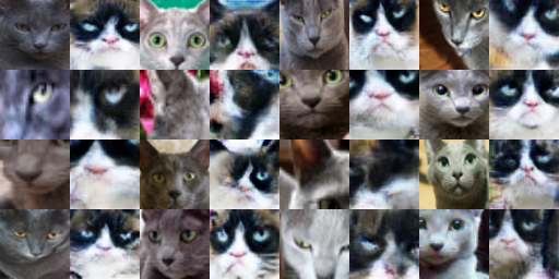 |
| Disciminator = Patch, Iterations = 10000; G_YtoX | 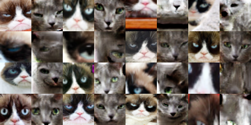 |
| Disciminator = Patch, Iterations = 10000, Cycle-consistency loss = True; G_XtoY |  |
| Disciminator = Patch, Iterations = 10000, Cycle-consistency loss = True; G_YtoX |  |
Following are the results for Apples-to-Oranges dataset :
| Configuration | Generated Samples (Apples and Oranges) |
|---|---|
| Disciminator = Patch, Iterations = 1000; G_XtoY |  |
| Disciminator = Patch, Iterations = 1000; G_YtoX |  |
| Disciminator = Patch, Iterations = 1000, Cycle-consistency loss = True; G_XtoY |  |
| Disciminator = Patch, Iterations = 1000, Cycle-consistency loss = True; G_YtoX |  |
| Disciminator = Patch, Iterations = 10000; G_XtoY |  |
| Disciminator = Patch, Iterations = 10000; G_YtoX |  |
| Disciminator = Patch, Iterations = 10000, Cycle-consistency loss = True; G_XtoY | 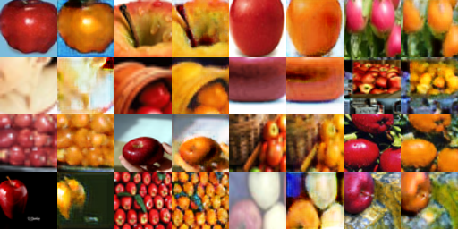 |
| Disciminator = Patch, Iterations = 10000, Cycle-consistency loss = True; G_YtoX |  |
From the above results for both, grumpy cats and apples to oranges, we see that without cycle consistency loss, the corresponding new domain image has the respective domain's features but it lacks the actual structure of the original domain. With cycle consistency loss, the corresponding new domain image has the respective domain's features and also the actual structure of the original domain. Hence, we can observe that the cycle consistency loss helps in learning better mappings between the domains.
| Configuration | Generated Samples |
|---|---|
| Disciminator = DC, Iterations = 10000, Cycle-consistency loss = True; Grumpy-Cats; G_XtoY |  |
| Disciminator = Patch, Iterations = 10000, Cycle-consistency loss = True; Grumpy-Cats; G_XtoY |  |
| Disciminator = DC, Iterations = 10000, Cycle-consistency loss = True; Apples-Oranges; G_XtoY |  |
| Disciminator = Patch, Iterations = 10000, Cycle-consistency loss = True; Apples-Oranges; G_XtoY |  |
The patch discriminator, in comparison to the DC-Discriminator, tends to generate images with higher realism due to its assessment on a patch-by-patch basis. This localized evaluation allows the patch discriminator to concentrate on intricate details and textures, resulting in more refined judgments of image fidelity. Our findings demonstrate that the patch discriminator yields crisper images, whereas the DC-Discriminator produces images with a slight decrease in sharpness, often exhibiting more blurring and artifacts.
5. Bells & Whistles : Samples using a pre-trained diffusion model
We use an off-the shelf pre-trained Diffusion model to generate some more grumpy cats!
Specifically, we use the "stable-diffusion-v1-4" model from the "diffusers" package from HuggingFace.
The prompt used is : "grumpy cat"
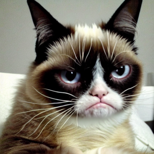
Fig26. Img 1
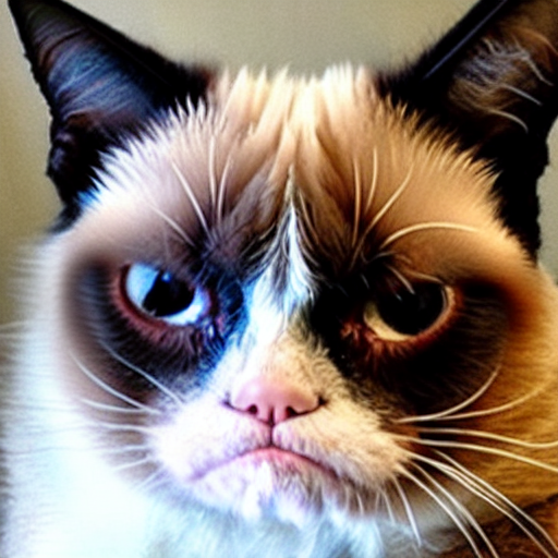
Fig27. Img 2
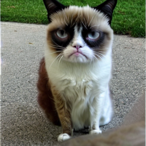
Fig26. Img 3
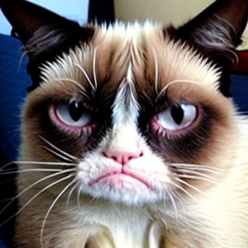
Fig27. Img 4
6. Bells & Whistles : Spectral-normalization for GAN stability
Training a GAN can be unstable, especially due to the fine balance between training the discriminator vs. the generator. We can use a weight normalization technique called spectral normalization to stabilize the training of the discriminator.

Fig31. DCGAN + Deluxe + DiffAug
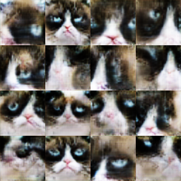
Fig32. DCGAN + Deluxe + DiffAug + SpectralNorm
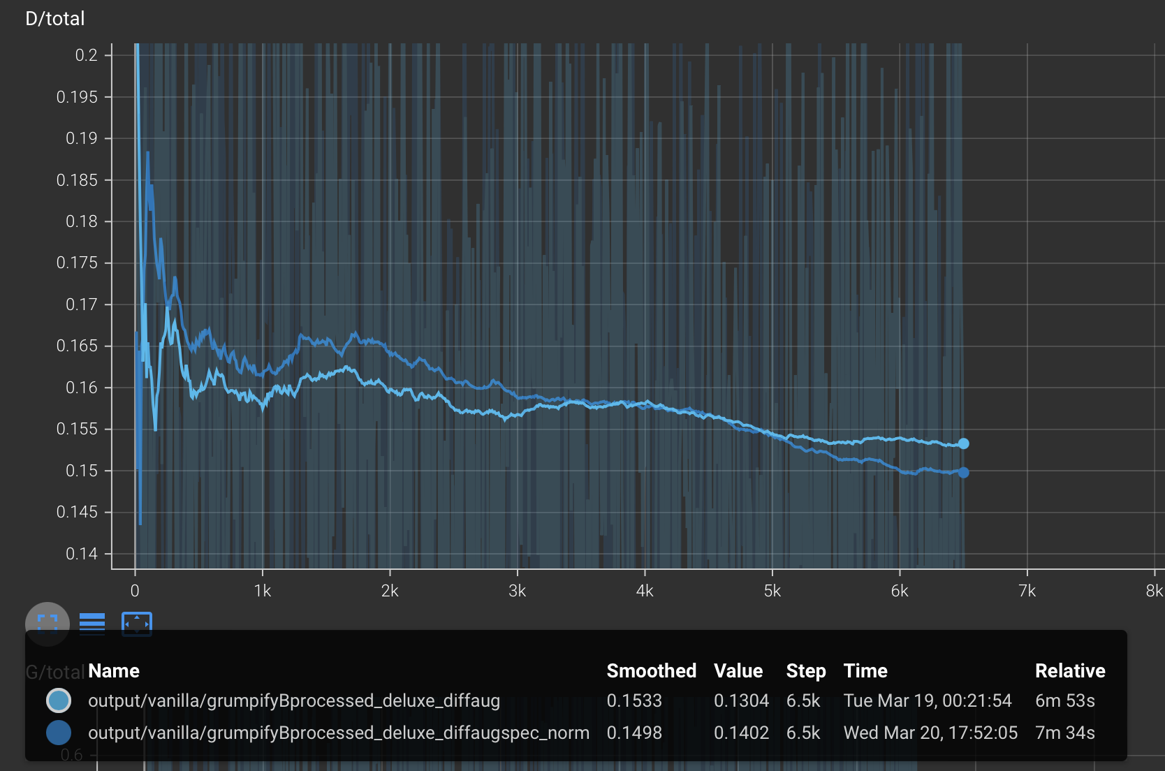
Fig31. DCGAN-discriminator + Deluxe + DiffAug : Learning curve (smoothing : 1)
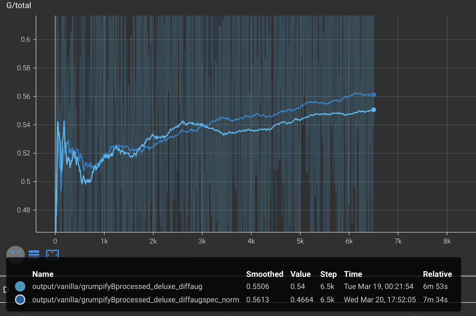
Fig32. DCGAN-generator + Deluxe + DiffAug + SpectralNorm : Learning curve (smoothing : 1)
Based on the training curves above, we see that the training is more stable (can be seen from the fluctuations in the curves). Furthermore, the results with spectral norm also look slightly better.
7. Bells & Whistles : Generate a GIF using GAN
GANs learn a distribution of the data and can generate new samples from this distribution. We can use this property to generate a GIF by interpolating between two images in the latent space of the generator. For this purpose, we perform linear interpolation between two random noise vectors and generate images at each step of the interpolation. We then combine these images to form a GIF.

Fig31. The cat is Grumpy-surprised!!


7. Bells & Whistles : Generate a GIF using GAN
GANs learn a distribution of the data and can generate new samples from this distribution. We can use this property to generate a GIF by interpolating between two images in the latent space of the generator. For this purpose, we perform linear interpolation between two random noise vectors and generate images at each step of the interpolation. We then combine these images to form a GIF.

Fig31. The cat is Grumpy-surprised!!
