

The goal of this assignment is to try out different image synthesis techniques to manipulate images in the latent space. To accomplish this, we invert a GANs model to find the latent space of an image this is done by optimizing the latent space to move towards the desired image. We then integrate masks/constraints into the mask to control the important regions of the image. Last of all, we finished a diffusion model implementation that can be used for an SDEdit-like modification of images, leveraging a DDPM-based scheduler.
After this, I implemented "bells and whistles" improvements:
Show some example outputs of your image reconstruction efforts using (1) various combinations of the losses including Lp loss, Preceptual loss and/or regularization loss that penalizes L2 norm of delta, (2) different generative models including vanilla GAN, StyleGAN, and (3) different latent space (latent code in z space, w space, and w+ space). Give comments on why the various outputs look how they do. Which combination gives you the best result and how fast your method performs.
The perceptual loss uses a pretrained vision network to guide the general features of the image. This is useful for ensuring that the image is not just a pixel-perfect reconstruction. I kept the loss at the default conv layer 5, so the loss maintains some low level feature representation, but can focus on high level features.


When perception loss is weighted particularly high, you see that we lose some important details, and the minimal loss appears to be just any cat that is approximately the right shape.
When the perception loss is weighted too small, the other loss (L1) takes over, and the image becomes more blurry. That said, some images are quite good (e.g. Perception loss of 1e-09). However, in general, I found that I was unable to reliably reproduce these good reconstructions and it is likely from a lucky random initialization.
In particular, I think that the 0.01 perceptual loss is the best. It had the most consistently reproducible good result, and it also continues to preserve some of the background. That said, 0.0001 and 1e-06 are also quite good.
With a perception weight = 1, the time was 27.638132572174072. The time for perception weight = 1e-9 was 27.181036949157715, a negligible difference. We are only changing one number, so this is expected.
The L1 loss is a pixel-wise loss that ensures that the image is a close match to the target. Ideally, using this loss for reconstruction should generate a pixel-perfect reconstruction. However, I found that this was not the case. In particular, the latent space that we are using does not possess all the information needed in an image, and as a result, I found that the L1 loss would still produce a blurry image. This makes some sense as the latent space does not encode all information, and instead the optimizer learns to minimize the pixel distance of certain images.


As the L1 loss increased, the image trended to a more consistently correct shape. In particular, if the L1 loss is too small, it seems a cat is placed in the correct position, but the shape of the cat does not quite line up with the reference image. If the L1 loss is large, it seems to still do decently well, but some blurriness starts to be introduced. Specifically, details like the eyes start to disappear.
I personally think that L1 weight of 10 holistically had the best match, but 1000 had a more aligned cat face. I'll use 10 for the rest of the experiments, but I later realized other target images were a little easier to work with and came back and generated some more examples for 1000.
The time for L1 weight = 100,000 is 27.4448561668396. The time for L1 weight = .001 is 27.111119031906128, a negligible difference. We are only changing a number so this is unsurprising.


This term appears to be optional and is only mentioned in the deliverables as an "and/or regularization loss that penalizes L2 norm of delta". I implemented this and ablated it anyway. Adding a regularizer will prevent the change in the latent space "delta" from being too large of a change. This means that adjusting this value will adjust how much the final image can change from the original image.


When regularization weight is too high, delta just goes to 0, and we have no changes. Once regularization gets low enough, overly large changes are prevented, so theoretically the changes should be more controlled. In my experimental results, this seems to translate to a less blurry image. That said, I found that the regularization hyperparameter has to be finetuned to each specific image, since each image has different features that changes the distance that has to be minimized.
For this image, the best values seems to be 0.001 or 1e-5. Generally, I either did not use the regularization term, or did another ablation to find the value to be used.
The time at weight = 10 was 27.36818528175354 and the time at weight = 1e-10 was 27.488969802856445, a negligible difference. We are only changing one number, so this is expected.


Unsurprisingly, the vanilla GAN model performed worse. We are not doing anything to augment the latent space, so this is expected.
The w and w+ latent spaces are augmented by being passed through a model mapping. The general appearance of the two images is similar as a result. However, the w+ latent space is more expressive and we expect it to be better. Personally, I would say that the (w+) latent space produces better results, based on the background and the the outline of the cat, but it is really close.
The time with vanilla z latent was 9.467675924301147, stylegan w latent was 27.556255340576172, and stylegan w+ latent was 27.459192276000977. The vanilla gan has the simplest implementation, so it is not surprising that it was the fastest. We may expect the w latent space to be faster than w+, but in reality, the code runs the tensors in the same passthrough, so the small difference in time is unsurprising.
For scribble to image, we implement a mask-based constraint to control the generation of the important regions of the image. It appears that the mask is a range based on intensity of a provided sketch. This mask is then used to weight the pixels of an image to produce a more controlled loss.
After some experimenting, I use the same weights for all of the following images:
The last (9th) image, was drawn by me. I will not be taking critiques at this time.


Experimentally, I found that sketches that utilized lines (0, 1, 6) rather than filled-in regions tended to be most successful when combined with a high L1 loss weight. This is because L1 loss ensures that the lines will show up in the final image output, for example, output 1 definitely has the lines of the sketch. However, if we want more realistic cats, a higher perception loss tends to be useful. My higher perception loss helps to retain the high level characteristics of the sketches, while retaining a more realistic cat. However, I found that these cats were more blurry if I mainly focused on the perception loss.
For denser, filled-in sketches (2, 3, 4, 5, 7, 8, 9), a high L1 loss was the most important loss. However, the sketches are not very realistic, so to get more realistic cats, I added the regularization loss. This reduced the amount of distortion/change a cat could have. The result is realistic cats for several images.
This combination did not do too well with fine-detailed lines like eyes or stripes. Higher regularization losses usually resulted in the cats not being "transformed" and instead it looked like the original image was masked out by the sketch. Higher perception losses would result in a blurry cat, which didn't really help with fine-details. Higher L1 loss tended to make the model try to match the lines exactly, which produces a weird face shape for the cat, which we can see happening in 1 and 6. Another problem for high L1 loss is that the cat may just exactly match the drawing. We can see something close to this starting to happen in image 3.
Overall though, I'm happy with how some images like cat 4 turned out. It's realistic while closely matching the sketch.
Lastly, I had a friend draw a cat as well. His drawing used a variety of colors and is a good way to test how the model handles color.
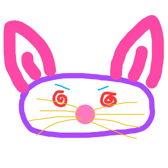

It seems when there is a bright color with high intensity, the color tends to transfer due to the high L1 loss that would result from this. That said, it seems that red/orange does not do as well as blue in this respect (as seen by the lack of red eyes for the cat). Perhaps cats have blue eyes, but there is nowhere in the latent space with red eyes. In general, the model does well with colors that it has experience with. When unnatural colors start showing up in unnatural places (red eyes, pink and purple outlines), the model ends up matching the outlines with a different, more natural color. This minimizes L1/perception loss and is presumably not too out of distribution for the latent space.
In this section, we implement a DDPM scheduler to control the diffusion model. We also implemented the code to noise and denoise from a certain step, which is the essence of the SDEdit.
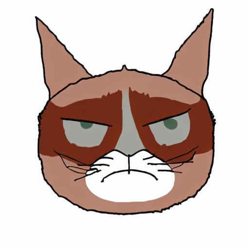
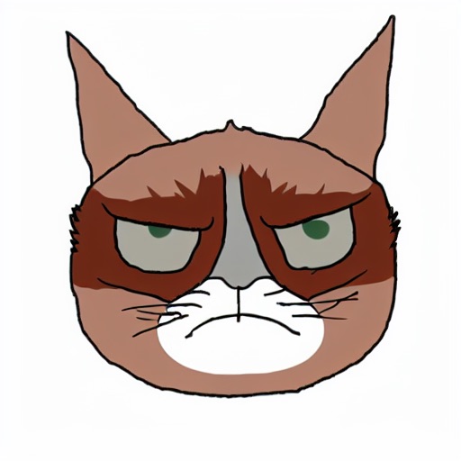
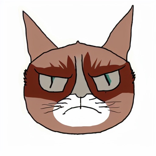
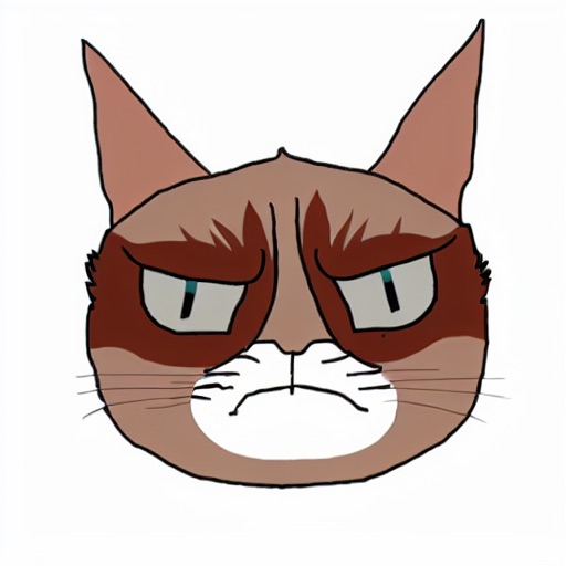
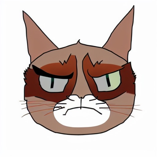
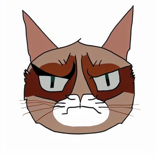
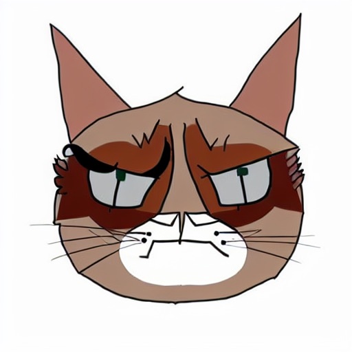
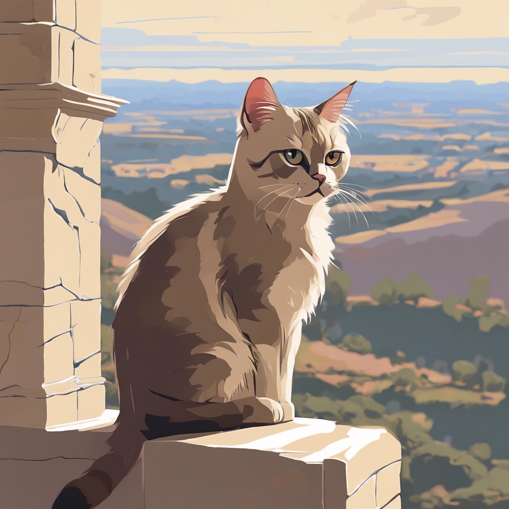
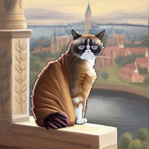
For my second image, I learned from my first attempt at drawing and decided to generate a second drawing of a cat from stability.ai's dreamstudio:
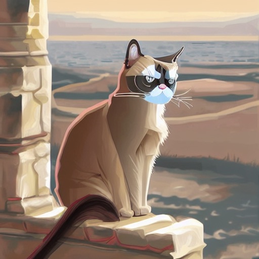
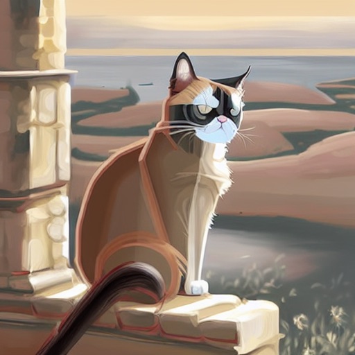
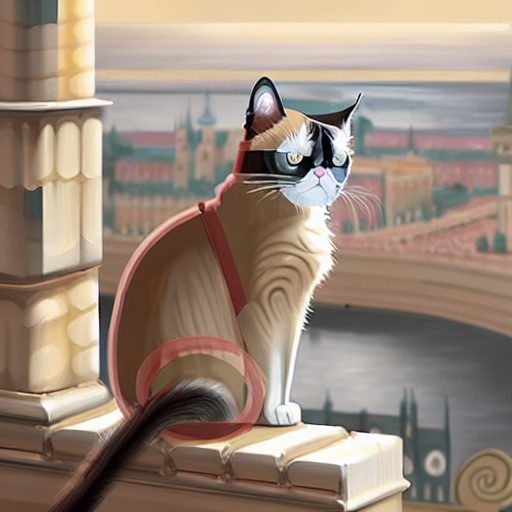
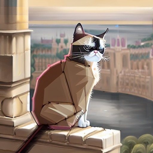
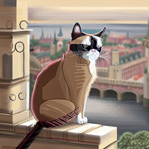

As expected, the higher the guidance value, the more impact the prompt "Grumpy cat reimagined as a royal painting" had on the output. In the first sketch, it seems that grumpy cat gets progressively grumpier as the guidance value increases. In the second sketch, it seems the term "royal" is impacting the background more and more as a kingdom develops.
An unintended effect is that the image has progressively more stylized lines as the guidance increases. I'm not sure why. Perhaps the model associated "painting" with lines?
For the first image, I arbitrarily chose guidance weight = 15.
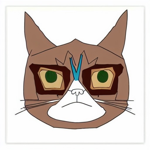
For the second image, I couldn't decied what the best looking guidance was, so I did both guidance weight = [15, 25].

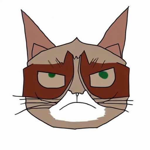
Guidance = 15

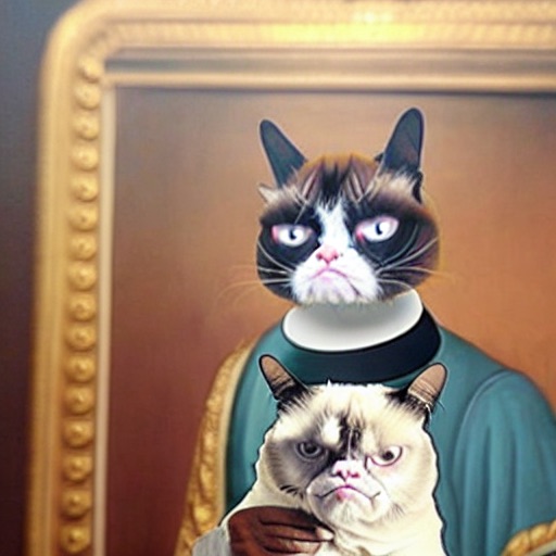
Guidance = 25

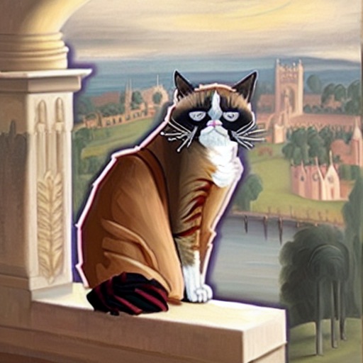

As expected, we can see that as the amount of denoising steps increases, we are getting more varied outputs. The image gets more noised and has more noising steps, so there is naturally more areas in the image where new details can be added.
DDIM's main innvoation is jumping to the predicted clean image, then renoising to the t-1 step. I implemented the formula from the paper. Their math formulation is slightly different from DDPM, so I just defined new variables that matched their notation rather than try to reuse the DDPM variables.
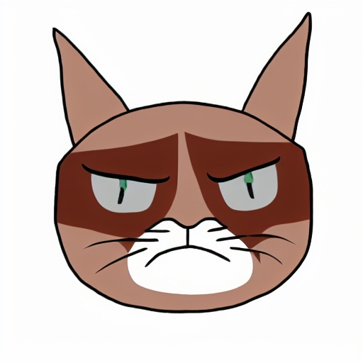
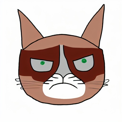
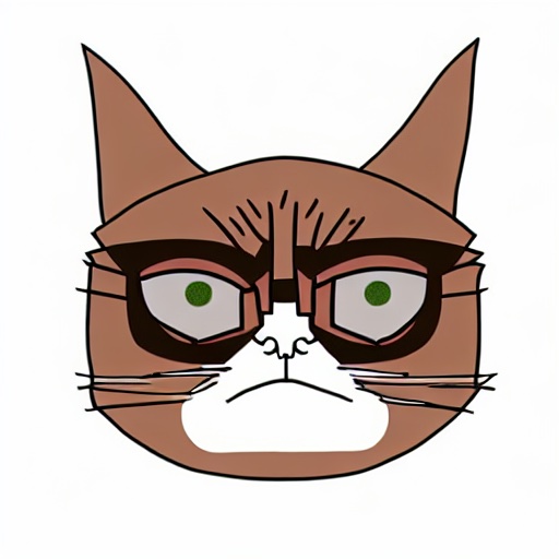
I think the main difference here is that we are just guiding the model towards a clean image, rather than making incremental denoising steps. As a result, DDIM's output is much smoother than DDPM's. I personally prefer DDIM's implementation.
For interpolation, I pretty much just find two latent codes, do a linear interpolation between them using convex combinations, then generate an image for each interpolation step. Each generated image becomes a frame in the gif.


