Thermal #3: Transient
heat transfer analysis of a rectangular slab
Introduction:
In this
example you will model a transient heat transfer. We will see how the
temperature field changes over time.
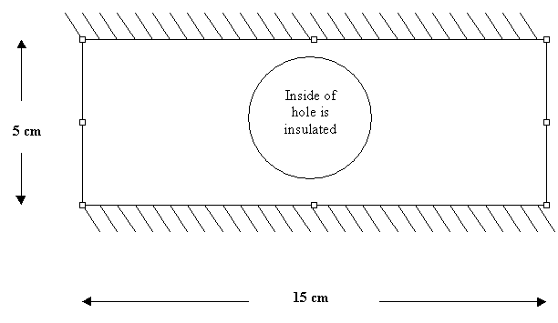
Physical Problem:
We
will model a rectangular slab with a hole in its center. It is
maintained at a constant temperature at one end and there is convective
heat transfer at the other end. The top and bottom of the slab are
insulated.
Problem Description:
 |
The slab is made of
material with density 5000 kg/m3. Its specific heat is 200
J/Kg K, and thermal conductivity is 5 W/m K. |
|
The bulk
temperature on the right of the slab is 293K, and the Film
Coefficient is 100 W/m2K. |
|
On the left side
the temperature on the boundary is 773K. |
|
Units: Use
S.I. units ONLY |
|
Geometry:
The hole in the center has a radius of 1cm. The hole is located at the
center of the slab. See figure for the rest of the dimensions.
|
|
Boundary conditions:
There is convection along the side walls. The top and the bottom walls
are insulated. The initial temperature of the slab is 293K
throughout. |
|
Objective:
 |
To plot the
temperature field in the slab 50 seconds after the boundary
conditions have been suddenly applied to the slab. |
|
To animate the
temperature field to see how it develops as time elapses.
|
|
|
You are required to
hand in print outs for the above. |
|
Figure:
|
|
IMPORTANT:
Convert all
dimensions and forces into SI units. |
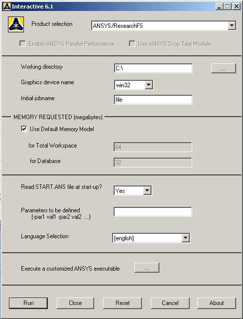
STARTING ANSYS
|
Click on ANSYS
6.1 in the programs menu. |
|
Select
Interactive. |
|
The following menu
that comes up. Enter the working directory. All your files will be
stored in this directory. Also enter 64 for Total Workspace and
32 for Database. |
|
Click on Run.
|
MODELING THE STRUCTURE
|
Go to the ANSYS
Utility Menu.
|
Click
Workplane>WP
Settings.
|
|
The following
window comes up: |
|
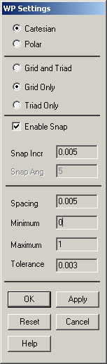
|
Check the
Cartesian and Grid Only buttons |
|
Enter the values
shown in the figure above. |
|
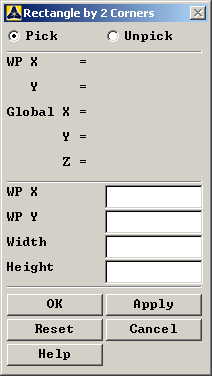
Go to
the ANSYS Main Menu and click
Preprocessor>Modeling>Create>Area>Rectangle>By 2 Corners
|
|
The following
window comes up: |
|
Now we will pick
the end points of the rectangles. |
|
First make the
outer rectangle of dimensions 15 cm X 5 cm (30 X 10 units on the
grid). |
|
Now got to
Preprocessor>Modeling>Create>Area>Circle>Solid Circle.
Create a circle of radius 1cm and with center at the center of the
rectangle. |
|
Now go to
Preprocessor>Modeling>Operate>Booleans>Subtract>Areas,
and subtract the circle from the rectangle by choosing the rectangle
first, then the circle. |
|
If you cannot see
the complete workplane then go to
Utility Menu>Plot Controls>Pan Zoom Rotate
and zoom out to see the entire workplane.
|
|
The model should
look like the one below: |

MATERIAL PROPERTIES
|
We need to define
material properties separately for steel, and the insulation
material. |
|
Go to the ANSYS
Main Menu and click
Preprocessor>Material Props>Material Models.
In the window that comes up choose
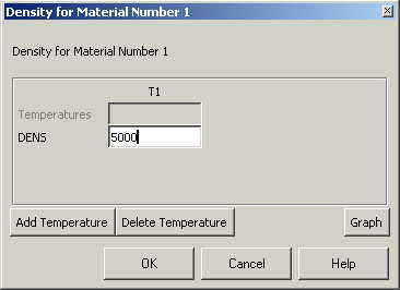
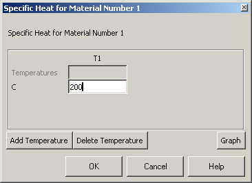
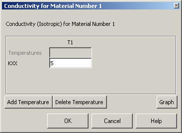
Density.
Put in 5000 for density. From the same window choose
Thermal>Specific Heat
and enter 200. From the same window choose
Thermal>Conductivity>Isotropic
and enter 5 for the thermal conductivity. The following
windows will appear as follows: |
|
Fill in the
appropriate values as shown in the figure above. Click OK. |
|
Now the material 1
has the properties defined in the above table. This represents the
material of the slab. |
ELEMENT PROPERTIES
|
SELECTING ELEMENT
TYPE: |
|
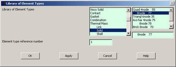
Click
Preprocessor>Element Type>Add/Edit/Delete...
In the 'Element Types' window that opens click on Add... The
following window opens. |
|
Type 1 in
the Element type reference number. |
|
Click on Thermal
Solid and select Quad 8node 77. Click OK. Close the
'Element types' window. |
|
So now we have
selected Element type 1 to be a thermal solid 8node element. The
component will now be modeled with thermal solid 8node elements. This
finishes the selection of element type. |
MESHING:
|
DIVIDING THE WALL
INTO ELEMENTS: |
|
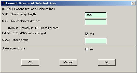
Go to
Preprocessor>Meshing>Size Controls>Manual Size>Lines>All Lines.
In the menu that comes up type 0.005 in the field for 'Element
edge length'. |
|
Click on OK. Now
when you mesh the figure ANSYS will automatically create a mesh, whose
elements have a edge length of 0.005m along
the lines you selected. |
|
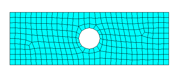
Now go to
Preprocessor>Meshing>Mesh>Areas>Free.
Pick the slab area and click OK. The meshed slab look like the
following: |
BOUNDARY CONDITIONS AND
CONSTRAINTS
|
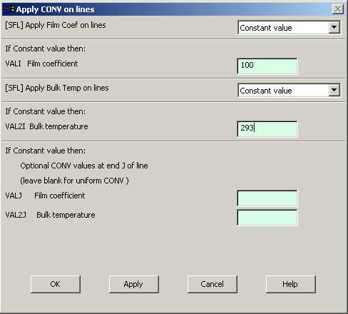
Go to
Preprocessor>Loads>Define
Load>Apply>Thermal>Convection>On Lines.
Pick the right line along the outer boundary. Click OK. The following
window comes up. |
|
Enter 100
for "Film Coefficient" and 293 for "Bulk Temperature" and click
OK. |
|
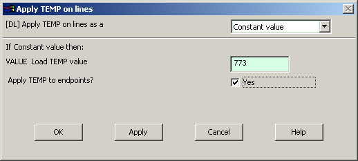
Go to
Preprocessor>Loads>Define Load>Apply>Thermal>Temperature>On Lines.
Pick the left line along the outer boundary. The following window
comes up. |
|
Enter the value of
the boundary temperature on the left edge of 773 K. |
|
Now the Modeling of
the problem is done. |
SOLUTION
|
Go to ANSYS
Main Menu>Solution>Analysis Type>New Analysis.
|
|
Select
Transient"and click on OK, then
select Full in the window that comes up. |
|
Go to
Main
Menu>Solution>Load Step Opts>Time/Frequency>Time-Time Step.
|
|
The following
window comes up: |
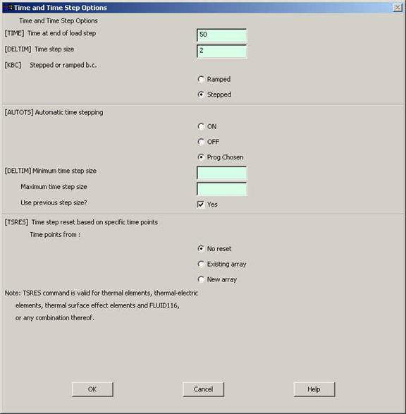
|
Fill in the values
as shown and click OK. |
|
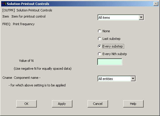
Now click
Solution>Load Step Options>Output Controls>Solution Printout.
|
|
The following
window comes up. Enter the values as shown and click OK. |
|
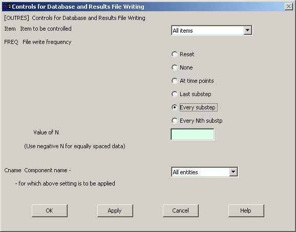
Now click
Solution>Load Step Options>Output Controls>DB/Results File.
|
|
The following
window comes up. Enter the values as shown and click OK. |
|
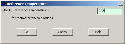
Now go to
Solution>Define Loads>Settings>Reference Temp.
|
|
The following
window comes up. Fill in the values shown and click OK. |
|
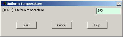
Go to
Solution>Define Loads>Apply>Thermal>Temperature>Uniform Temperature.
|
|
The following
window comes up. Enter the values as shown and click OK. |
|
Now go to
Solution>Solve>Current LS.
|
|
Wait for the
solution to get done. |
|
Close the "Stat
Command" window. |
|
Now the solution is
done. |
POST-PROCESSING
|
Plotting the
temperature field after 50 secs.
|
|
Go to ANSYS Main
Menu and click on
General Postprocessing>Read Results>By
Load Step.
The following window will come up. |
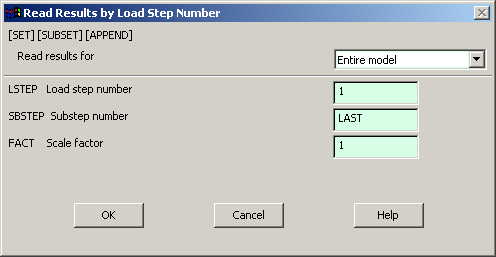
|
Enter values as
shown and click OK. |
|
Now go to
General Postprocessing>Plot
Results>Contour Plot>Nodal Solution.
|
|
The following
window comes up. Enter the values as shown and click OK. |
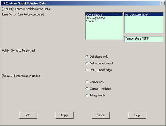
|
The temperature
distribution looks something like the plot below. |

|
Animating the
development of the temperature field |
|
Go to
Utility Menu>Plot Controls>Animate>Over Time.
The following window comes up. Enter the values as shown and click OK:
|
