We will model the turbine as a disk with blades fixed on it ('blisk'=bladed disk). The inner radius of the hub is 10 cm, outer radius is 40 cm, blade length is 20 cm, blade width is 5 cm, and the thickness is 2.5 mm

Material: Assume the structure is made of steel with modulus of elasticity E=210 GPa and has a Poisson ratio of 0.3 and density of 7.21e3 kg/cubic meter.

Boundary conditions: The blisk is fixed around the inner diameter of the disk.

Loading: The blisk is not loaded.

Objective:

	To determine first three family of modes.
	To animate the mode shape of the first 3 modes.
	You are required to hand in print outs for the above. You don't have to hand in the animation files but you will have to give at least 3 captured frames of the animation for each of the three modes.

Figure:

Click on ANSYS 6.1 in the programs menu.

Select Interactive.

The following menu that comes up. Enter the working directory. All your files will be stored in this directory. Also enter 64 for Total Workspace and 32 for Database.

Click on Run.

We will model one quarter of the blisk and then reflect it to create the complete blisk.3

Go to the ANSYS Utility Menu.

	Click Workplane>WP Settings.
	The following window comes up:

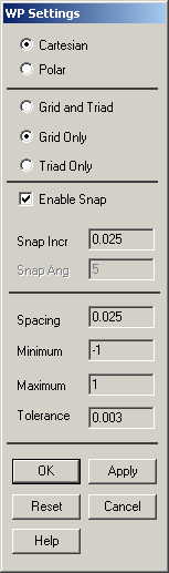
Check the Cartesian and Grid Only buttons

Enter the values shown in the figure above.

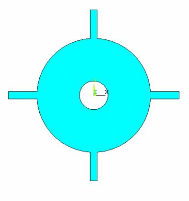
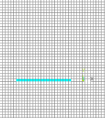
The following is the quarter blisk we will model first:

Go to the ANSYS Main Menu Preprocessor>Modeling>Create>Areas>Rectangle>By 2 corners.

Select the two corners for the horizontal rectangle and click Apply. Remember the rectangles (blades) have a thickness half the actual thickness since we are modeling only a quarter of the blisk.

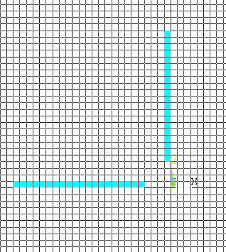
Now similarly create the vertical rectangle.

Now we will create the quarter disk. Go to Preprocessor>Modeling>Create>Areas>Circle>Partial Annulus. The following window comes up:

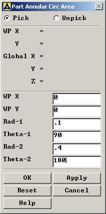
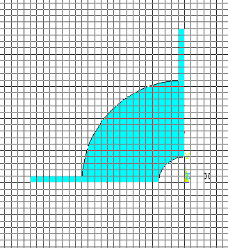
Enter the values as shown and click OK. The model looks like the one below:

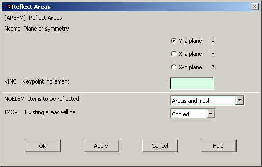
Now we will reflect the areas we have created about the YZ plane and then all the areas about the XZ plane. Go to Preprocessor>Modeling>Reflect>Areas. Click on "Pick All". the following window comes up:

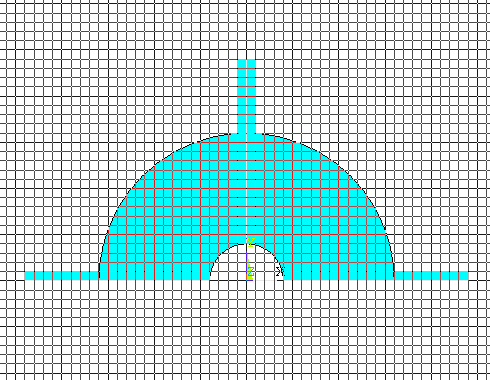
Select the YZ plane and say OK. The figure will look like the following:

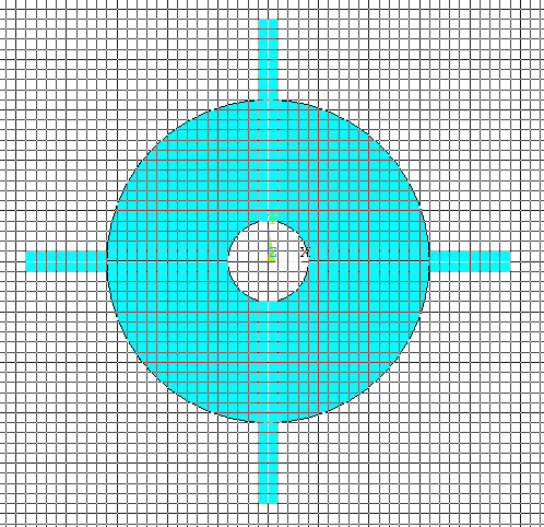
Now repeat the same process and reflect the whole figure about the XZ plane. The figure will look like this now.

Now we will add the areas up. Go to Preprocessor>Modeling>Operate>Booleans>Add>Areas.

In the window that comes up click "Pick all".            

Go to the ANSYS Main Menu

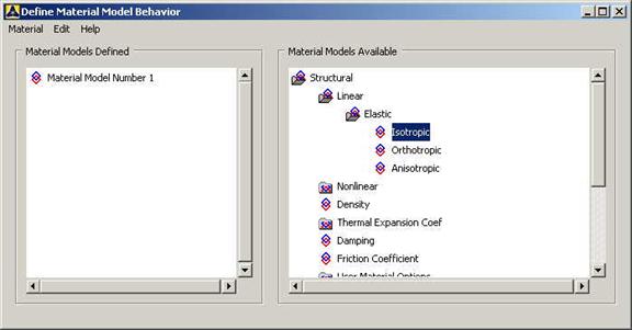
Click Preprocessor>Material Props>Material Models.  In the window that comes up, select Structural>Linear>Elastic>Isotropic.

Enter 1 for the Material Property Number and click OK. The following window comes up.

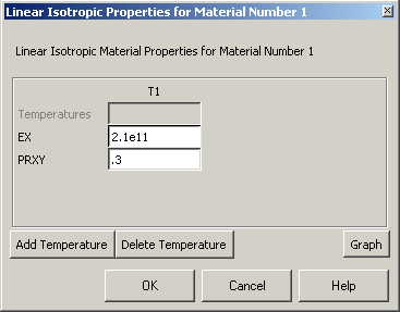
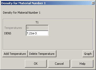
Fill in 2.1e11 for the Young's modulus and 0.3 for minor Poisson's Ratio.  From the Material Model window, select Structural>Density and enter 7.21e3 for the density. Click OK.

Now the material 1 has the properties defined in the above table. We will use this material for the structure.

SELECTING ELEMENT TYPE:

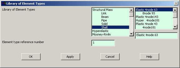
Click Preprocessor>Element Type>Add/Edit/Delete... In the 'Element Types' window that opens click on Add... The following window opens:

Type 1 in the Element type reference number.

Click on Structural Shell and select Elastic 4node 63. Click OK. Close the 'Element types' window.

Now we need to define the thickness for this element.

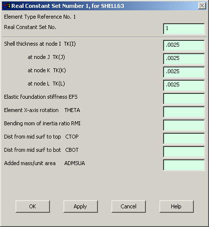
Go to Preprocessor>Real Constants>Add/Edit/Delete...

In the "Real Constants" dialog box that comes up click on Add

In the "Element Type for Real Constants" that comes up click OK. The following window comes up.

Fill in the relevant values and click on OK.

We have now defined the thickness of the element.

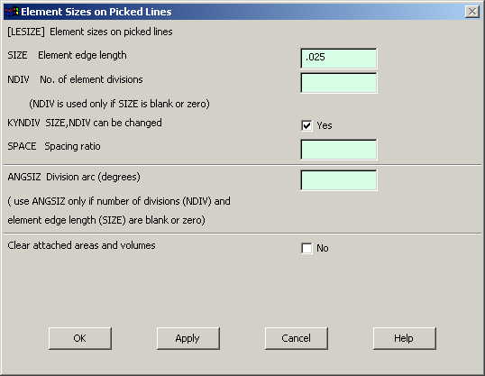
Go to Preprocessor>Meshing>Size Controls>Manual Size>Lines>Picked Lines. Pick all the lines on the outer boundary of the figure and click OK.

In the menu that comes up type 0.025 in the field for 'Element edge length'.

Click on OK.

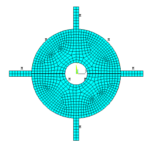
Now go to Preprocessor>Meshing>Mesh>Areas>Free.

Click "pick all" in the "Mesh Areas" dialog box. The meshed model looks like this.

Now the blisk is divided into Shell elements.

APPLYING BOUNDARY CONDITIONS

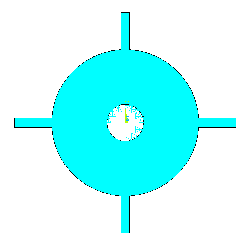
The blisk is fixed around the inner diameter of the disk.

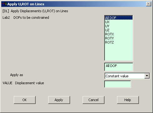
Go to Main Menu Preprocessor>Loads>Define Loads>Apply>Structural>Displacement>On Lines.

Select the lines on the inner circumference of the disk and click OK. The following window comes up:

Select All DOF and click OK. 

The model now looks like this:

Now the Modeling of the problem is done.

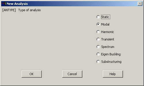
Go to ANSYS Main Menu>Solution>Analysis Type>New Analysis. The following window comes up:

Select Modal and click on OK.

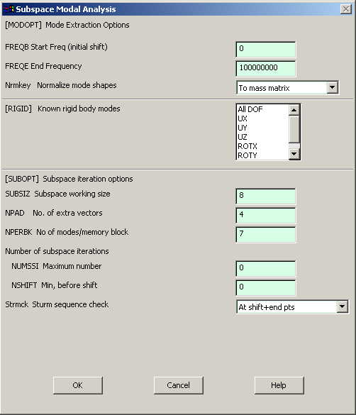
Now go to Main Menu>Solution>Analysis Type>Analysis Options. The following window comes up:

Enter the values shown in the window above and click OK. The following window comes up.

Enter 100000000 for the End Frequency.  Then Click OK.

Go to Solution>Solve>Current LS.

Wait for ANSYS to solve the problem.

Click on OK and close the 'Information' window.

To list the first three frequencies, go to Main Menu>General Postprocessing>Results Summary. The following window will be displayed:

To animate the mode shapes, go to Main Menu>General Postprocessing>Read Results>First Set.

Go to Utility Menu>Plot Controls>Animate>Mode Shape. The following window will come up:

Select the required animation: in this case Deformed Shape and click OK.

The animation will be similar to the ones below. (Don't capture images from these files, they are not the solutions. Just similar to solutions.)

	ANIMATION 1
	ANIMATION 2
	ANIMATION 3

To plot the deformed shape, go to Main Menu>General Postprocessing>Read Results>First Set.

Now in the same window go to Plot Results>Contour Plot>Nodal Solution. The following window comes up:

Select DOF solution, and select USUM.

Check the Def + undeformed button.

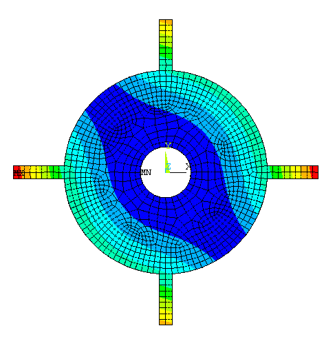
Click on OK. The contour plot will look similar to the figure below.