Synthesizing Optimal Parallel Collectives via SAT
1/23/2024
Parallel collectives are the building blocks of parallel programs that enable communication between processes. These are critical to distributed GPU workloads, with as much as 11-63% of ML training being spent waiting for collectives to execute (Sapio et al, 2020). The design space is overwhelming and unintuitive, making it difficult to find optimal implementations. In this project, we present a SAT-based approach to synthesizing optimal parallel collectives. We show that our approach can synthesize optimal implementations for a variety of collectives and topologies.
This project was conducted two years ago with wonderful collaborators Ranysha Ware, Margerida Ferreira, Surabhi Singh, and Ruben Martins. This work follows up on the incredible "Synthesizing Optimal Collective Algorithms" (Cai et al, 2021). Though we enjoyed this project, we did not publish it since we didn't provide a major methodological contribution. This (very late) writeup is intended to be a friendly introduction to the beautiful problem formulated by the original work, as well as a simpler and faster solution for practice. You can find our codebase at this github link.
Background
Topology
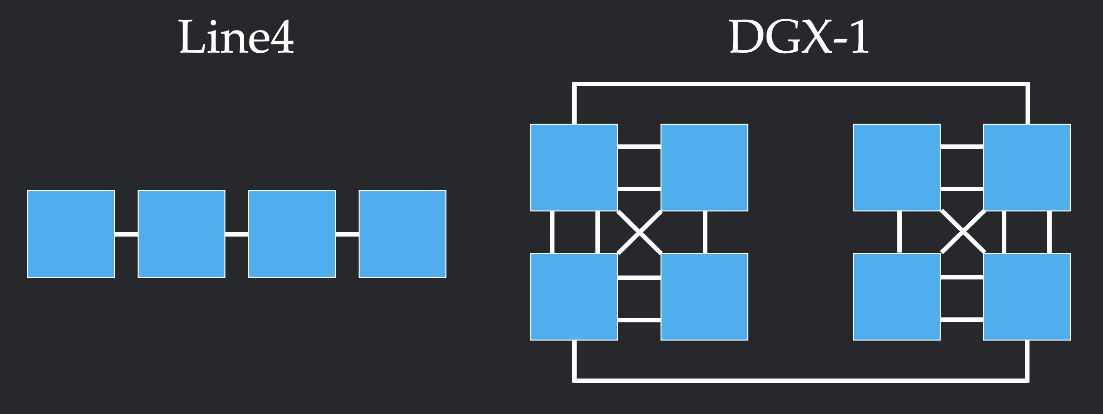
We start by considering a system with nodes that each contain some chunks of data. A network topology is a set of links where each link connects two nodes. A node can send a copy of their chunk to another node via a link between them. When a node sends data through a link, it must respect the bandwidth constraints of the link, meaning that the total number of chunks passing through the link at any given time must be less than or equal to the link's capacity. Below, we show two examples of network topologies. In the left, we see a simple Line4 topology with 4 nodes that are each connected to their neighbor(s) by link constraints of capacity 1. On the right we can see the more complicated NVIDIA DGX-1 topology.
Collectives
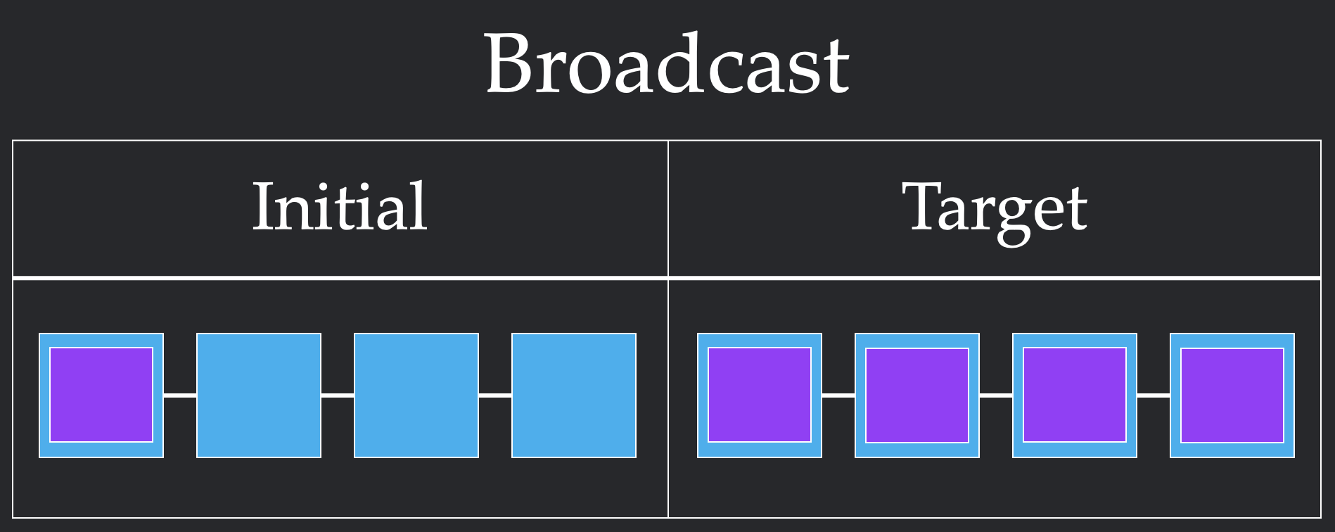
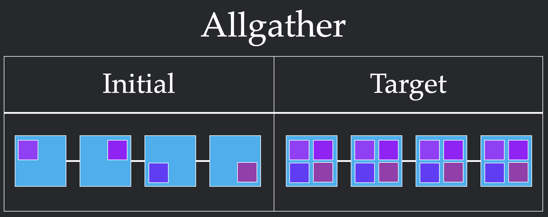
Given a topology, we can now specify how we want to move data via collectives. Each collective specifies a pre-condition where the data starts and a post-condition where the data must end up. In the following figure, we show examples of two different collectives: Broadcast, which expects to share all the data from one node to every other node, and Allgather, which expects all data to be shared to every node. Users build algorithms via these primitives, while systems provide an implementation that meets the user's specification. You can find more examples of collectives at this link.
Cost of an Implementation
What does a successful collective implementation look like? A full algorithm consists of steps, each of which consists of rounds. In one round, multiple nodes can send each other multiple chunks, as long as the combination of all sends meets the bandwidth constraints. One step can contain as many of these rounds as it would like, as long as the order of the rounds doesn't matter. Computationally, a round represents the time it takes to send the chunk over the link, while a step represents the amount of time spent opening and closing connections between chunks sending data to each other. These definitions are really difficult to understand, so let's walk through two different ways to solve 2 chunk Broadcast for Line4.
In the first implementation, we first send both chunks from node 1 to node 2. Since the bandwidth constraint is 1, this requires two rounds to send both chunks. However, since these rounds themselves can be parallelized, this only requires 1 step. We repeat this from node 2 to node 3, and node 3 to node 4, to get a final solution that requires 6 rounds and 3 steps.
In this second implementation, we first send a single chunk from node 1 to node 2. This requires one round. From here, we stagger our sends, sending one chunk from node 1 to node 2 and one from node to node 3 in the same round. We repeat this to get all of our chunks across. This more unintuitive pattern requires 4 rounds which is more than the previous 3 rounds. However, it only takes 4 steps, since we cleverly parallelize sends to respect the bandwidth constraint.

In our formalization, we will refer to the round count as bandwidth and the step count as latency. Different physical systems have different times for opening connections and sending chunks, which will determine whether its better to use the first or second implementation. For the rest of this article, we measure the speed of a collective via its latency and bandwidth in this toy model.
Problem Statement
Problem Statement: Can we efficiently synthesize the optimal implementations for collectives?
Previous work has answered affirmatively, showing that we can use SMT tools to find optimal collectives. In this work, we will offer a simple SAT encoding of the problem which is orders of magnitude more efficient than their implementation.
We first decompose our problem into two aspects: synthesis and optimization. We first provide an interface which, for a topology, collective, step budget, and round budget, will return a successful implementation or a proof that it is impossible to do so. Then, we will use this synthesizer to find an implementation which optimizes a desired metric of performance (i.e bandwidth-optimal).
Synthesizing with SAT
We will assume we are given a topology with \(N\) nodes, \(C\) chunks of interest, and \(E\) links (where links with non-unit constraints are decomposed into multiple links of constraint 1). For a given round budget \(R\) and step budget \(S\), we try all \(\binom{R-1}{S-1}\) possible partitions of the \(R\) rounds into different steps and check if any of these partitions is possible. To check if a partition is possible, we first denote time points ranging from time \(0\) (before step 1) to time \(t\) (after step \(t\)). We can now assign a boolean variable \(p_{c,n,t}\) to denote whether chunk \(c\in [C]\) is present at node \(n\in[N]\) at time \(t \in [0, S]\). Then, we assign a boolean variable \(s_{c,e,t}\) to denote whether chunk \(c\in[C]\) is sent over link \(e\in[E]\) between time step \(t-1\) and \(t\) for \(t\in[S]\). For a specific time step \(i\), we multiply the number of links by the rounds in that step \(R_i\) to encode multiple rounds happening simultaneously.
Given this parameterization, we need to find an assignment of the boolean variables that is valid according to the topology and successfully implements the collective: if we find a satisfying assignment, we have a valid algorithm of bandwidth \(R\) and latency \(S\), and otherwise, we have proven no such algorithm exists.
We now use the fact that a SAT problem is precisely finding a satisfying assignment of boolean variables under first-order logic constraints. For our problem, we need to encode many such constraints--as an overview, constraint types 1-2 enforce the collective is met, 3-4 enforce valid sends, 5 enforces capacity constraints by merging the rounds in a step, and 6-7 are redundant but lower the search space. Note that we can use cardinality encodings to encode sum constraints.
- The pre-condition of the collective is met (\(p_{c,n,0}\) is 1 if and only if a chunk of data starts there according to the collective)
- The post-condition of the collective is met (\(p_{c,n,s}\) is 1 only if a chunk of data must end there according to the collective)
- Sending requires the chunk is at the source (for all \(t > 0\), \(s_{c, (n, n'), t} \Longrightarrow p_{c, n, t}\))
- A new chunk requires a send (for all \(t > 0\), \(p_{c, n', t} \land \neg p_{c, n', t-1}\) \(\Longrightarrow\) \(\bigvee_{(n, n')\in E}s_{c, (n, n'), t-1}\))
- Capacity constraints are respected (\(\sum_{c\in[C]} s_{c, e, t} \leq b \cdot R_i\))
- If a chunk appears, it never goes away (for all \(t > 0\), \(p_{c, n, t-1} \Longrightarrow p_{c, n, t}\))
- The same chunk never needs to be sent more than once (\(\sum_{t\in[S]} s_{c, e, t} \leq 1\))
Phew. We encode these logical constraints in PySAT and run the CaDiCaL solver to see whether there exists a valid collective.
Optimizing the runtime
With this powerful validity predicate implemented via SAT, we can now search for different solutions. For example, if we wanted the bandwidth optimal solution (minimize round count) we simply try 1 step 1 round, 2 step 2 round, etc until we find a satisfying solution. To find the latency optimal solution (minimize step count), we can try 1 step infinite round, 2 step infinite round, etc until we find a satisfying solution. More interestingly, we consider Pareto optimal solutions, or those that can beat every other solution on at least one axis (conversely, for solutions that aren't Pareto optimal, there exists at leats one strategy that dominates it in both resources). We propose an efficient strategy to find the Pareto frontier, or all Pareto optimal solutions (implemented in our repo). With this, a practitioner can look through the set of Pareto optimal solutions for which works best for their hardware.
Results
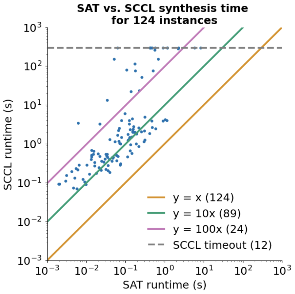
Enough yapping, does our method actually find the optimal solutions? Inspired by the original paper, we consider trying to implement {Allgather, Gather, Broadcast, Alltoall, Allreduce} on the topologies {DGX-1, DGX-2, AMD8, Line, Ring, FullyConnected, Hypercube3}. We will try to find the bandwidth or latency optimal solution for 1-5 chunks. We will also give both algorithms a 5 minute timeout. When trying our method out on these problems compared to the original paper, we find that we are orders of magnitude faster, as indicated by the following plot. As such, our simpler SAT encoding offers advantages over SCCL implemented in SMT!
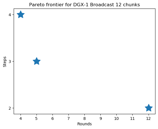
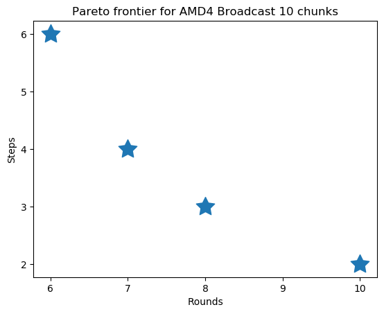
We also demonstrate our Pareto frontier search algorithm. Below, we show how we can find the full frontier for two different collectives.
Thank you for reading, and feel free to reach out with any questions or thoughts!