Convex Geometry for Computers

8/13/2023

Today we will be covering how to convey (high-dimensional and non-convex) geometry to computers. Specifically, we will be discussing how computers can efficiently represent shapes, how they can quickly optimize functions over such shapes, and how to bound this optimization for approximation and verification. Along the way, we'll see how convexity is such an important and beautiful condition, allowing for strong approximations to problems that are otherwise impossible. This intro is best suited for somebody who knows what convexity means,though we briefly introduce these concepts for the uninitiated.

What is Convexity?

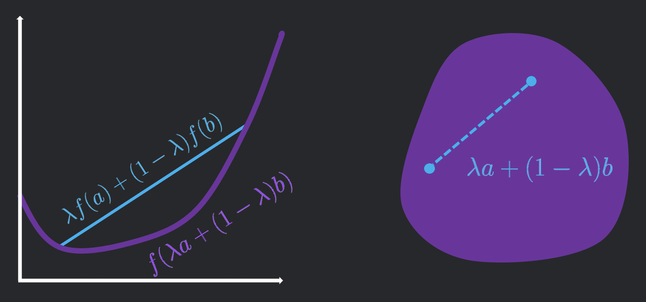
We define a convex combination of two points $a$ and $b$ as $\lambda a + (1-\lambda)b$ for any $\lambda \in [0, 1]$. This is best visualized as any point along the line between $a$ and $b$, and there is a natural extension to more points as a linear combination with non-negative coefficients that sum to $1$.

We can visualize a convex function $f$ as a "bowl facing upward". More concretely, for any two points $a, b$ in the domain of $f$, we have the "convex combination of the outputs is greater than the output of the convex combination of the inputs", or

\[\forall a, b, \lambda \in [0, 1], f(\lambda a + (1-\lambda)b) \geq f(\lambda a) + f((1-\lambda)b).\]

A convex set $S$ is a shape such that it contains every convex combination of any two points $a, b \in S$, or

\[\forall \lambda \in [0, 1], \forall a \in S, \forall b \in S, \lambda a + (1-\lambda) b \in S .\]

The extreme points of a set are points in the set that can not be expressed as a convex combination of other points in the set. For a polygon, this would be the vertices.

Figure 1: On the left, we picture a convex function satisfying the linear upper bound property. On the right, we picture a convex set containing all of it's convex combinations.

Representing Convex Sets

Defining the Convex Hull

Representing sets in general is impossible (we can't even represent every real number on a computer!), but convex sets generally have some nice structure which makes them easier to represent. We start by defining a really cool operator called the convex hull.

The Convex Hull of a set $S \subseteq \mathbb{R}^d$, written as $\text{Conv}(S)$, has the following equivalent definitions.

The set of all convex combinations of subsets of $S$
The smallest convex set containing $S$
The set of all convex combinations of the extreme points of $S$
The intersection of all half-spaces that contain $S$

From these, you can pick your favorite definition to show that $S$ is convex iff $\text{Conv}(S) = S$. Importantly, definitions 3 and 4 give us nice ways to represent convex sets

The V-representation, which constitutes the extreme points of the set
The H-representation, which constitutes the half-spaces that contain the set

Geometric Duality

For different sets, we care about using different representations of our set. For some fundamental examples, let's consider $\ell_p$ balls in dimension $d$ (defined by $\{x \in \mathbb{R}^d: \|x\|_p \leq 1\}$).

Figure 2: Visualization of $\ell_p$ balls

The $\ell_1$ ball has $2d$ extreme points and is contained by $2^d$ half-spaces.
The $\ell_{\infty}$ ball has $2^d$ extreme points and is contained by $2d$ half-spaces.
The $\ell_2$ ball has infinite extreme points and infinite half-spaces that contain it, so we should not use the V or H representations.

From the above, it seems like we would want to use the V-representation for $p=1$, the H-representation for $p=\infty$, and neither for $p=2$. We also run into a cute "flip" between what's needed for $p=1$ and $p=\infty$. Is it just a coincidence? Actually, it's an instantiation of a more general Duality Transform, which takes a shape and inverts it over the unit sphere. Specifically, given a set $S$, construct the set $S^* = \{q : \langle q, p \rangle \leq 1, \forall p \in S\}$. By convexity, this is equivalent to $\{q : \langle q, p \rangle \leq 1, \forall p \in \text{ExtPts}(S)\}$. Note that this corresponds exactly to an intersection of half-spaces, specifically $|\text{ExtPts}(S)|$ of them. Moreover, through expanding the definitions we can see that the dual of the dual is the original shape, or that $S^{**} = S$.

We observe that the $\ell_1$ ball and the $\ell_{\infty}$ ball are duals of each other. This explains why their vertex and half-space counts are flipped—it's because the duality transform swaps each extreme point for a half-space and each half-space for an extreme point! Also since the $\ell_2$ ball is its own's dual, this is why it has the same number of faces and vertices.

Convex Functions over Convex Sets

Many of the important problems in computer science can be phrased under optimization, or finding the best valid point with respect to an objective function. In it's most general instantiation, we write it in the format of a "Mathematical Program" as follows.

$$\begin{aligned} &\text{maximize} && f(x) \\ &\text{subject to} && x \in S \end{aligned}$$

With the tools from the previous section, we can rewrite $x \in S$ as a set of inequalities represented by $g(x) \leq 0$. For simplicity, I am omitting many simple generalizations such as expressing equalities via inequalities, expressing minimization as the negation of maximization, multiple inequalities, etc. For a general choice of objective function $f$ and constraint set $S$, this problem is intractable since optimization is generally very difficult. However, for some well-behaved choices, this problem becomes feasible and often very efficient. The art comes in formulating the $f$ and $S$ of interest for the domain, representing it a computer-friendly manner, and then writing or using the correct algorithm to solve your specific program.

Let's start by assuming that both $f$ and $S$ are convex. We know that for a convex set, every point can be expressed as a convex combination of the extreme points. Therefore, by the convexity of $f$, we know that any maximum to the objective function must lie at one of the extreme points. Therefore, if the function has very few extreme points, then our task is really easy.

Bounding Convex Functions over Convex Sets

Finding the precise answer to an optimization problem is really difficult. In many cases, we are actually more interested in bounding the optimization problem, giving some lower or upper bounds. For a minimization problem, the value at any feasible point serves as an upper bound, since the minimum of the objective function can not be greater than the value at all of the feasible points. In practice, when the set is well-behaved, one can efficiently get bounds by doing Projected Gradient Descent, or using gradient descent while staying inside the constraint set to find tighter upper bounds. In fact, for convex problems, this technique is guaranteed to converge.

Lower bounding a minimization problem is much more complicated since its hard to say something that's simultaneously true for all of the points in the constraint set. However, its often this property that makes lower bounds so useful—of the objective function says something about safety or violating a property, a lower-bound can certify that all points are safe.

Lagrange Duality

To efficiently provide tight lower bounds, we introduce the technique of Lagrange duality. Let's start by considering the program which we want to lower bound.

$$\begin{aligned} &\min_x && f(x) \\ &\text{s.t.} && g(x) \leq 0 \end{aligned}$$

The current problem is that we don't know where $g(x) \leq 0$ so we try to remove this constraint by folding it into the optimization problem. We can do this introducing a Lagrange multiplier $\lambda$, as shown in the following program.

$$\begin{aligned} &\min_x \; \max_{\lambda\geq 0} \; f(x) + \lambda g(x) \end{aligned}$$

In this new program, it seems like there are no constraints, so it might be surprising that its equivalent to our original program. However, let's consider this min max formulation as a two player game, where the outer player (who we'll name Minnie) selects a value of $x$ and the inner player (who we'll name Maxie) then selects a value of $\lambda$ based on this choice. If Maxie selects an $x$ such that $g(x) > 0$, then Minnie will select a $\lambda$ arbitrarily large and drive the entire optimization problem to $\infty$. This is at odds with Minnie's goal of minimizing the objective value, so Minnie will only select values of $x$ such that $g(x) \leq 0$. Interestingly, this renders Maxie's best strategy to always set $\lambda = 0$ since any other value can only hurt Maxie and help Minnie. Therefore, the two programs are equivalent!

Even though these problems are equivalent, the new problem is not any easier to solve. For our next trick, we observe that we can switch Minnie and Maxie to lower bound the value of the problem above by the problem below!

$$\begin{align} &\max_{\lambda\geq 0} \; \min_x \; f(x) + \lambda g(x) \end{align}$$

This is a direct consequence of the minimax theorem, which is briefly proven below.

\[\begin{aligned} h(x', y') &\geq \min_{x} h(x, y') && \text{(true for all $x', y', h$ by definition of min)} \\ \max_{y} h(x', y) &\geq \min_{x} h(x, y') && \text{(true for all $x', y', h$ by definition of max)} \\ \max_{y} h(x', y) &\geq \max_{y} \min_{x} h(x, y) && \text{(true for all $x', h$ by picking the best y')} \\ \min_{x} \max_{y} h(x, y) &\geq \max_{y} \min_{x} h(x, y) && \text{(true for all $h$ by picking the best x')} \\ \end{aligned}\]

We consider this problem the dual of the original problem, which we refer to as the primal. By our inequalities above, we've proven that the dual of a minimization problem always serves as a lower bound to the primal. Before we dive into the beauty of duality, let's work through a simple example.

$$\begin{aligned} &\left[\min_x x_1^2 + 2x_2^2 \;\text{ s.t. }\; x_1 + x_2 \geq 1\right] \\ &\geq \left[\max_{\lambda \geq 0} \min_x x_1^2 + 2x_2^2 - \lambda x_1 - \lambda x_2 + \lambda \right] && \text{(Lagrange duality)} \\ &= \left[\max_{\lambda \geq 0} -\frac38 \lambda^2 + \lambda \right] && \text{(min solved by $x_1 = \frac{\lambda}{2}, x_2 = \frac{\lambda}{4}$)}\\ &= \frac{2}{3} && \text{($\lambda = \frac{4}{3}, x_1 = \frac{2}{3}, x_2 = \frac{1}{3}$)}\\ \end{aligned}$$

The above shows that the original quadratic program is lower bounded by $\frac{2}{3}$. But before we discuss that, let's look at some of the beautiful properties of the process of Lagrange duality.

Dual is always convex: Note that the inner problem is a minimum of functions linear in $\lambda$ for every choice of $x$. Since a minimum of linear functions is always concave, the outer objective is always concave in $\lambda$. Since optimizing a concave problem under convex constraints $\lambda \geq 0$ is a convex problem, the dual is always convex regardless of how gnarly the original problem is.
Closed form in $x$: Frequently, after the swap of Maxie and Minnie, the inner minimization problem will have a closed form in $x$ due to the lack of constraints. This allows us humans to aid the computer by deriving the optimal solution and removing the inner minimization problem.
Lower bound for all $\lambda$: By definition of max, our lower bound holds for any choice of $\lambda$. Therefore, even if we do not find the $\lambda$ which solves the outer optimization problem, our choice can give a sound lower bound, and we can now apply heuristic techniques like Projected Gradient Descent on $\lambda$ to get sound lower bounds for safety!

These properties make Lagrange duality an excellent computational tool to lower bound optimization problems! However, one natural concern is how tight these bounds are; it would be a little too magical for us to get tight lower bounds for every problem. A sharp eye would observe that for the earlier quadratic program, the solution to the dual is the solution to the primal! When the dual and the primal have no "gap", we have Strong Duality. When there is a gap, we say that we have Weak Duality. For example, all linear programs (linear objective and constraints) meet strong duality. Through visualizing convex duality (which I'll add here another day :)), we can get a sense for why strong duality holds for all convex problems and why the dual of a convex relaxation is the convex relaxation of the dual.

I hope you enjoyed the introduction to how computers represent shapes and optimize functions as well as why convexity is such a fundamental aspect of computational geometry. Please reach out if there are any questions or errors!