Lower Diversity Accelerates Convergence for Regression
\( \def\truedist{{\overline{X}}} \def\allset{{\mathcal{X}}} \def\truesample{{\overline{x}}} \def\augdist{\mathcal{A}} \def\R{\mathbb{R}} \def\normadj{\overline{A}} \def\pca{F^*} \def\bold#1{{\bf #1}} \newcommand{\Pof}[1]{\mathbb{P}\left[{#1}\right]} \newcommand{\Eof}[1]{\mathbb{E}\left[{#1}\right]} \newcommand{\xquery}{x_{\text{query}}} \newcommand{\yquery}{y_{\text{query}}} \newcommand{\ypred}{\hat{y}} \newcommand{\prompt}{P} \newcommand{\functionfamily}{\mathcal{F}} \newcommand{\promptfamily}{\mathcal{P}} \newcommand{\predloss}{\mathcal{L}} \newcommand{\Normal}{\mathcal{N}} \newcommand{\normalpdf}[1]{\varphi\p{#1}} \newcommand{\prob}{{\mathbb{P}}} \newcommand{\identityd}{I_d} \DeclareMathOperator*{\argmax}{arg\,max} \DeclareMathOperator*{\argmin}{arg\,min} \newcommand\bSigma{{\mbox{\boldmath$\Sigma$}}} \newcommand{\wcont}{w_{\text{cont}}} \newcommand{\wdisc}{w_{\text{disc}}} \newcommand{\wcontopt}{w^*_{\infty}} \newcommand\wdiscopt[1]{w^*_{{#1}}} \newcommand{\wmixopt}{w^*_{\text{mix}}} \newcommand{\weightdist}{\mathcal{D}} \newcommand{\dist}[1]{\weightdist_{#1}} \newcommand{\contdist}{\dist{\infty}} \newcommand\discretedist[1]{\dist{{#1}}} \newcommand{\finetunedist}{\dist{\text{finetune}}} \newcommand{\finetuneprob}{p_{\text{finetune}}\p{X, y}} \newcommand{\numsamples}{T} \newcommand{\mixturedist}{\dist{\text{mix}}} \newcommand{\sequencesamples}{x_1, y_1, \ldots, x_k, y_k} \newcommand{\trueposterior}{g(X,y)} \newcommand{\modelposterior}{g_{\theta}(X,y)} \newcommand{\modelscaledposterior}{g_{\theta}(X,\gamma y)} \newcommand{\promptstrat}{s} \newcommand\pb[1]{{\left[ #1 \right]}} \newcommand\inner[2]{{\left< #1, #2 \right>}} \newcommand{\E}{{\mathbb{E}}} \newcommand\p[1]{{\left( #1 \right)}} \newcommand\sW{{\mathcal{W}}} \)5/20/2024
We will consider training transformers to perform linear regression (originally considered by the visionary work of Garg et al, 2022). For Gaussian data, it is Bayes-optimal to perform ridge regression. However, we find that making the data less diverse can find ridge regression before eventually converging to the Bayes-optimal solution for the less diverse data. Magically, the model learns ridge regression much much faster training on the less diverse data compared to the full Gaussian data. This is perhaps the most surprising empirical phenomenon I have ever encountered, and I have very little intuition for why this happens ever since I found it fifteen months ago (documented in Appendix C.3 of Kotha et al, 2023). I would like to share this magic and would be especially grateful if somebody can help me understand why it happens.
Setup
Data format
(This setup closely follows Section 2 of the aforementioned paper). We are interested in learning functions \(f \in \functionfamily\) that map inputs \(x \in \mathbb{R}^d\) to outputs \(y \in \mathbb{R}\). Inspired by previous works, we focus on linear regression for noisy data, where every function is given by \(f_w\colon x \mapsto \inner{w}{x}\) for a fixed \(w \in \R^d\). We are given a set of samples \(S\) of variable length \(k\) from \(0\) to maximum length \(40\) such that
\begin{align} S = \left\{(x_1, y_1), \ldots, (x_k, y_k)\right\}, \label{eq:samples} \end{align}
with \(y_i = f_w(x_i) + \epsilon_i\) and \(\epsilon_i \sim \Normal(0, \sigma^2)\). From this, a model estimates the output \(\yquery\) for a given input \(\xquery\). We will refer to an instance from our function class $f_w$ as a task, and when it is clear from context, we will refer to tasks by the associated weight vector $w$. In this section, all inputs will be sampled from the normal distribution via $x_i \sim \Normal(0, \identityd)$.
Training an auto-regressive model
We consider auto-regressive models $T_\theta$ that take in a sequence of tokens, each in $\R^d$, to produce a real-valued output. For samples $S$ generated under $w$, we feed $T_{\theta}$ the prompt $\pb{\sequencesamples, \xquery}$ (every $1$-dimensional token is right-padded with $d-1$ zeroes) and take its output as a prediction of $\yquery$. When appropriate, we will refer to the $x_i$'s in the prompt as $X \in \R^{k\times d}$ and the $y_i$'s as $y \in \R^{k}$. We train and evaluate $T_\theta$ with respect to a weight distribution $\weightdist$ via the quadratic loss
\begin{align} \label{eq:in-context} \predloss(\theta, \weightdist) = \sum_{k=0}^{40} \underset{ \substack{ x_i \sim \Normal(0, \identityd) \\ w \sim \weightdist \\ \epsilon_i \sim \Normal(0, \sigma^2) } }{\E}\pb{\p{T_{\theta}\p{\pb{\sequencesamples, \xquery}} - \yquery}^2}. \end{align}
by sampling a fresh batch of $x, w, \epsilon$ each step. Under quadratic loss, the optimal output is
\begin{align}\E\pb{f_{w}(\xquery) + \epsilon \mid X, y} = \langle \E\pb{w \mid X, y}, \xquery \rangle\end{align}
Therefore, it suffices to recover the expectation of the weight's posterior distribution over the data. For our model, we use a 22.4 million paramater GPT-2 style transformer. For more experimental details, refer to Appendix C.8 of the original paper.
Task Distributions
Gaussian Task Distribution is solved by Ridge Regression
Prior work assumes weights are sampled from a Gaussian prior \(\contdist = \Normal(0, \tau^2\identityd)\), which we will refer to as the "continuous distribution". In this case, the Bayes optimal predictor performs ridge regression:
\begin{align}\wcontopt(X, y) = \E\pb{w \mid X, y} = \p{X^{\top} X + \frac{\sigma^2}{\tau^2}\identityd}^{-1}X^{\top}y.\end{align}
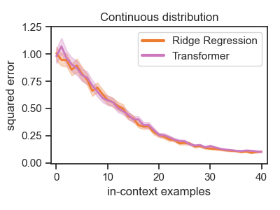
As noted in prior work, for most values of $\tau, \sigma$, a converged transformer's predictions closely match the Bayes optimal predictor when evaluated on weight vectors from the same Gaussian prior. We replicate this for $\tau = 1$ in Figure 1, left.
Discrete Task Distribution is solved by Discrete Regression
We now consider training over a "fixed" set of weights with the distribution $\discretedist{N}$ sampling $w$ uniformly from $\sW_{N} = \{w_1, \ldots, w_N\}$. We refer to this as the "discrete distribution". With this new prior, ridge regression is no longer optimal. The Bayes optimal estimator for $\discretedist{N}$ is:
\begin{align} \wdiscopt{N}(X, y) &= \frac{\sum_{w \in \sW_N}w \normalpdf{(y - Xw)/\sigma}}{\sum_{w \in \sW_N}\normalpdf{(y - Xw)/\sigma}}, \end{align}
where $\normalpdf{\cdot}$ is the density of the standard multivariate normal distribution (derivation in Appendix B.1). We refer to this estimator as discrete regression.
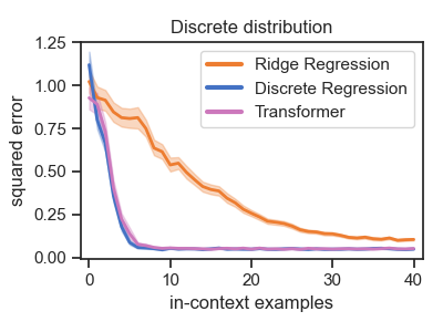
After training for sufficiently many steps on $\discretedist{64}$, we find that the Transformer achieves the same loss as the Bayes-optimal estimator $\wdiscopt{64}$, clearly outperforming ridge regression on the fixed set of weights (Figure 1, right).
The Magic
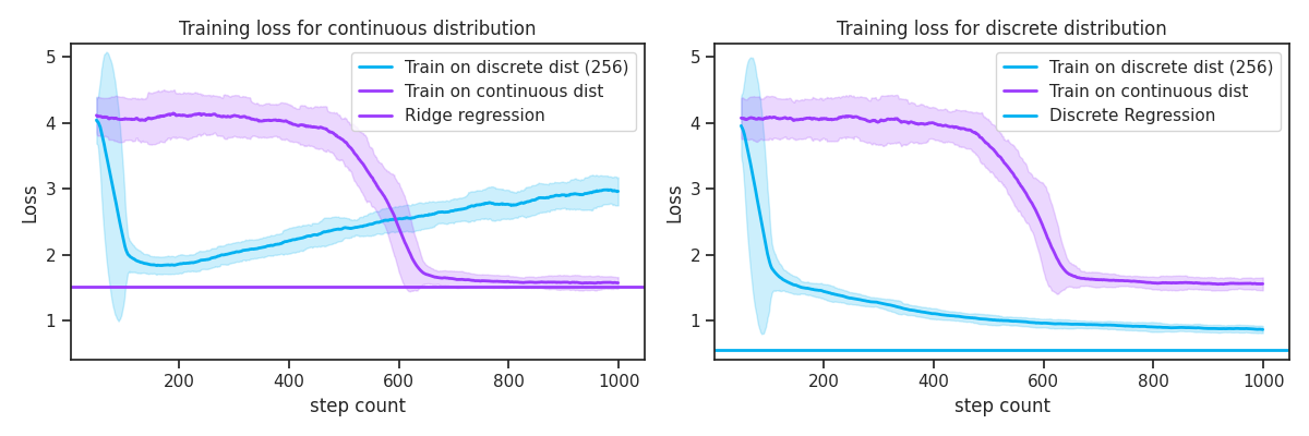
So far, we've seen how training for long enough converges to optimal solution. However, the magic comes from the training trajectory. Though training on the discrete distribution eventually converges to discrete regression, we actually learn ridge regression!! This can be seen in Figure 2. What's even more magical is that we reach ridge regression much much faster by training on the discrete distribution compared to the continuous distribution. It is incredibly surprising that training on a less diverse data distribution improves the speed of convergence to the true generalizing solution.
Effect of Task Count
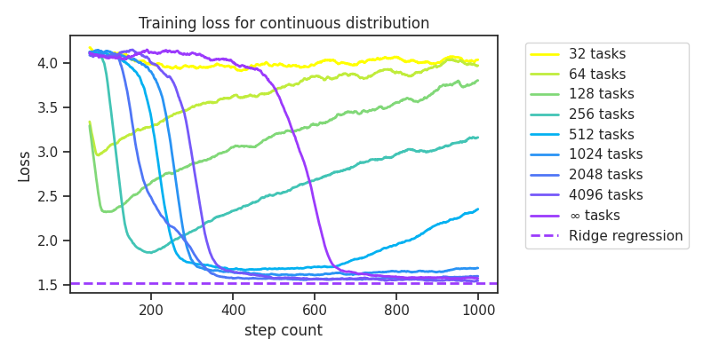
Obviously, this depends on the number of tasks, which we plot in Figure 3. If there are too few tasks (e.g. 32), then the model never learns ridge regression along the way to discrete regression. If there are too many tasks (e.g. 4096), then its effectively equivalent to training on the full gaussian distribution and there is no increase in speed of convergence. However, our experiments reveal a sweet spot in the middle where the model quickly learns righe regression before losing it for discrete regression. There is some variance for running over a fixed task count, but I find that this trend holds robustly over many reruns.
Next Steps
As of writing this (May 2024), I have very little understanding as to why this phenomenon occurs. I can believe that ridge regression is encountered along the way due to a simplicity bias towards the simpler solution of ridge regression. However, I have absolutely zero understanding of why the training is so much faster, so robustly across many experiments. To better understand, I first want to see how far I can simplify the setting. Is this true for mean estimation instead of linear regression? Is this true for different architectures and smaller models? This will hopefully uncover what factors are important for this phenomenon. It would be awesome to build a fine-grained understanding of how diversity affects the speed and quality of training, especially in a way that generalizes to real training.
Thank you for reading, and feel free to reach out with any questions or thoughts!