Paper Analysis: A Universal Law of Robustness via Isoperimetry
1/3/2023
Today we're going to explore a beautiful probabilistic result connecting the mathematical hardness of data distributions to the robustness of neural networks that fit them. The original paper, Bubeck and Sellke, 2021, is very well-written so please defer to them for the full math, setup, details, and related work. In this post, we'll spend time on the assumed mathematical background, a proof sketch to distill the essence of the argument, and a discussion on the broader significance to robustness.
Theorem - Informal
On realistic data distributions and assumptions, there exists an upper bound of the robustness of any function with low loss, where the bound is looser for more parameters.
Background
Lipschitz constant: A function \(f\) is \(L\)-Lipschitz over a norm \(\|\cdot\|\) if for all points \(x_1, x_2\) in its domain, it satisfies the following implication. $$\|x_1 - x_2\| \leq c \Longrightarrow \|f(x_1) - f(x_2)\| \leq Lc$$ This says that when two inputs are close, the outputs are also close, highlighting the smoothness of such a function. Therefore, a low constant says that a function has a low "stretch" factor, compared to non-Lipschitz functions which are capable of egregiously overfitting any training data.
Robustness: Robustness is the study of ML in settings where the test distribution is not equivalent to the train distribution. Though there are many specifications of robustness, this paper focuses on how the model's classification reacts to small perturbations in the input space, or in other words, the Lipschitz constant! The Lipschitz constant is one of the simplest characterizations of the robustness of a model, which offers advantages and disadvantages (which we get into at the end of this article).
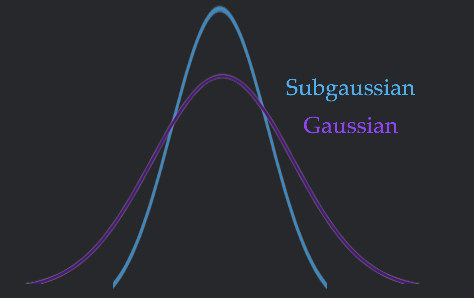
Subgaussian: A random variable \(X\) is \(C\)-subgaussian if \(\mathbb{P}\left[|X| \geq t\right] \leq 2e^{-t^2/C}\). This is equivalent to the variable being more tightly concentrated than a Gaussian random variable.
Isoperimetry (the daunting definition)
A \(d\)-dimensional data distribution satisfies \(c\)-isoperimetry if for any bounded \(L\)-Lipschitz function
\(f :
\mathbb{R}^d \to \mathbb{R}\), $$\mathbb{P}\left[|f(x) - \mathbb{E}[f]| \geq tL\right] \leq
2e^{-\frac{dt^2}{2c}}$$
In less symbols, this means that a distribution is always \(c\)-subgaussian under the scaled image of a
Lipschitz
function (the \(-\mathbb{E}[f]\) centers the output around the mean and the \(tL\) represents the stretch of the
\(L\)-Lipschitz function). In more English, this means that a data distribution is tightly concentrated. Since a
more concentrated distribution can not be classified by a function of low Lipschitz constant, this definition
captures some inherent difficulty in the data distribution.
Isoperimetry is a well-studied property and it has been proved that Gaussians with small corruptions and
low-dimensional manifolds satisfy the requirements. This means that under the manifold hypothesis, real-world
data distributions satisfy isoperimetry.
Theorem - Less Informal
Now that we've taken the time to understand the background, we have the language to formulate the mathematical result! Suppose the following preconditions are met
- The function class \(\mathcal{F}\) maps \(\mathbb{R}^d \to \mathbb{R}\), is Lipschitz in its \(p\) real parameters, and has weights bounded by \(\text{poly}(n, d)\)
- The input distribution satsifies \(c\)-isoperimetry
- The data distribution has nonzero noise, or \(\sigma^2 := \mathbb{E}[\text{Var}[y|x]] \geq 0\)
With high probability over the sampling of \(n\) data points \((x^{(i)}, y^{(i)})_{i\in[n]}\), \(\forall f \in \mathcal{F}\)
$$\frac{1}{n} \sum_{i=1}^n\left(f\left(x^{(i)}\right)-y^{(i)}\right)^2 \leq \sigma^2-\epsilon \Longrightarrow \operatorname{Lip}(f) \geq \widetilde{\Omega}\left(\epsilon \sqrt{\frac{n d}{p}}\right)$$
This should match the English of the informal claim: a model with low loss has a parameter-based lower bound on the Lipschitz constant!
Proof Sketch
In this sketch, we consider the case where the loss must be \(0\) (following the paper's lovely exposition). Since most of the intuition and the mathematical instruments are demonstrated in this case, we do not discuss the concentration inequalities necessary to generalize this result to the main result.
One function fitting one point
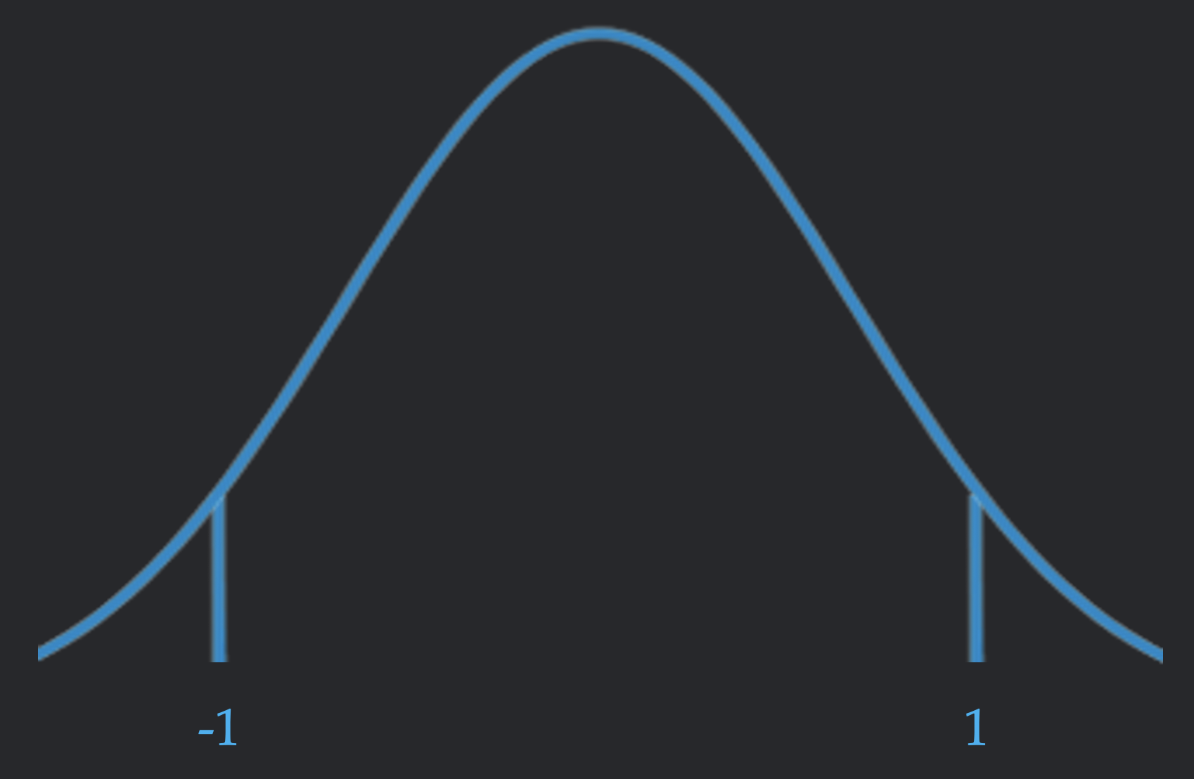
To understand if there's a low-Lipschitz function that fits the data, we first consider if an arbitrary function in the function class can fit the data. Suppose we randomly labelled a \(1\)-isoperimetric input distribution with \(\pm 1\) labels. By looking at the definition of isoperimetry, the probability that the output of the model is close to \(-1\) or \(+1\) is low; a perfect label assignment happens with probability \(\leq 2e^{-\frac{d}{2L^2}}\). Since lining up with \(-1\) or \(+1\) are disjoint events, one of these events has at most half this probability, or \(\leq e^{-\frac{d}{2L^2}}\). We'll call this a "difficult" label.
It is important to note that this upper bound is stronger when the Lipschitz constant is lower; as the function class gets less expressive, its much harder for a function to fit an arbitrary point.
One function fitting all points
We can prove that with high probability, our random labelling of the data will have many \(+1\) labels and many \(-1\) labels; for mathematical convenience, lets say that each label has at least \(\frac{n}{13}\) inputs. Therefore, at least \(\frac{n}{13}\) of the points are difficult. To fit all the points, we need to fit the difficult labels, which happens with probability \(\leq e^{-\frac{nd}{26L^2}}\) (since each label is assigned independently). Therefore, the probability of any function fitting all of the points is low.
Any function fitting all points
This bound looks great for an individual function but when there are infinitely many functions in the class
(which is the case for weights in \(\mathbb{R}^p\)), we can't use a union bound to prove the non-existence of a
low Lipschitz function...
To deal with this, we can bring in the neat geometric tool of the \(\epsilon\)-net. On a high level, to prove
something about an infinite set, we construct a finite cover of the space such that every element can be
well-approximated by some points in the cover. When this condition holds, one can prove that a property that
holds for the finite cover approximately holds for all of the points in the covered space.
Now, we can take the first and only step that concerns deep neural networks. It happens to be that a Lipschitz
neural network is also
Lipschitz in its weight vector (the vector \(\in \mathbb{R}^p\) that contains each weight). When
we bound the weights, we can set up a cover in the weight space. By union-bounding the event of a function
fitting all the points (which we proved was small), we can show that its very difficult for any function in the
cover to fit all the points. This
shows that its difficult for any function approximated by the \(\epsilon\)-net to fit all the points. This
concludes the proof sketch.
Robustness? (My thoughts)
The theoretical contributions are quite impressive since they provide an incredibly general proof that more
parameters are necessary for a smooth fit to the data (along with a matching upper bound). Isoperimetry feels like a natural choice for analyzing the property of interest, which is the Lipschitz constant. Since the paper has a
great discussion of its details, extensions, and implications, I will not belabor this point.
That being said, it is worth going back to our very first definition: the Lipschitz constant. Though this
constant is the most mathematically convenient method of defining robustness,
how much meaning does it directly carry? In the case of adversarial robustness, it seems like the answer is not
that much. The paper claims to address the worst-case robustness of ML. However, when we look at the state of
the art defenses, they happen to offer true worst-case robustness despite a high Lipschitz constant.
The most performant adversarially robust algorithm is randomized smoothing. In this defense, one applies a
small Gaussian
corruption to the input before asking the model to classify it. Though an ensemble of these corruptions can
(with high probability) provably defend against attacks (Cohen
et
al, 2019), such a model is not Lipschitz, showing how the
Lipschitz constant can not explain randomized models.
In the case of provably safe defenses (i.e. models that can be proved to have a consistent output in an
\(\epsilon\)-ball around an input), many verifiers actually utilize the Lipschitz constant. However, it is
important to note that they use the local Lipschitz constant, or the tightest Lipschitz constant that
holds in an \(\epsilon\) vicinity of an input point. Even if a network has a globally high Lipschitz constant,
it can have a very low Lipschitz constant in the region local to data points (Hein and Andriushchenko 2017). In fact, even
SOTA
empirically robust models explicitly optimize for this metric rather than global smoothness (Qin et
al, 2019). Therefore, its unclear
that the global Lipschitz constant discussed here provides any barrier to worst-case robustness.
Summary
Isoperimetric data is tightly concentrated. Its unlikely that an arbitrary function solves an arbitrary label of
this data. Its unlikely an arbitrary function solves many labels. Its unlikely any function in a finite
collection solves many labels. A finite collection of functions can approximate all functions of interest. Its
unlikely any function in the function class solves many labels. Though this result shows low paremeters implies
high Lipschitz, high Lipschitz implies not robust is a tenuous connection that requires more care.
Thank you for reading, and feel free to reach out with any questions or thoughts!