Optimal Experimental Design with Compute Constraints
\( \def\truedist{{\overline{X}}} \def\allset{{\mathcal{X}}} \def\truesample{{\overline{x}}} \def\augdist{\mathcal{A}} \def\R{\mathbb{R}} \def\normadj{\overline{A}} \def\pca{F^*} \def\bold#1{{\bf #1}} \newcommand{\Pof}[1]{\mathbb{P}\left[{#1}\right]} \newcommand{\Eof}[1]{\mathbb{E}\left[{#1}\right]} \newcommand{\Normal}{\mathcal{N}} \newcommand\p[1]{{\left( #1 \right)}} \newcommand{\sumc}{\sum_{i\in[n]} c_i} \newcommand{\sumsqc}{\sum_{i\in[n]} c_i^2} \newcommand{\sumec}{\sum_{i\in[n]} e^{c_i}} \)5/28/2024
After toying with a simple regression problem, I found an intersection with the field of optimal experimental design (seen in the wilderness thanks to Hashimoto, 2021 and Ruan et al, 2024). I was curious about a simple question: what inputs should we select to best estimate the underlying parameters of a system? In this post, we will solve this for linear regression. We will then apply these simple principles to optimally fit scaling laws under various budget constraints. The optimal solution is NOT to equally space the inputs, and I hope you find the correct solutions as surprising as I did.
Linear Regression
We start with a simple problem: how should we pick inputs for linear regression? We will consider a setup where there is a ground truth weight vector \(w \in \R^d\) where each choice is equally likely (flat prior). Everytime we submit an input \(x^{(i)} \in \R^d\), we will recieve an output \(y^{(i)} \in \R\) which is equal to \(w^{\top} x + \epsilon\) for \(\epsilon \sim \Normal(0, \sigma^2)\). This corresponds to getting a noisy estimate of the true label for any chosen input. We will stack \(n\) such points as \(X \in \R^{n\times d}\) and $y \in \R^n$.
Optimal Estimator
Before determining optimal inputs, we will think about a prerequisite question: for inputs $X$ and outputs $y$, what is the optimal estimate of the underlying weight? To determine this, we first construct the posterior, the distribution of the weight conditioned on the observed data.
\[ \begin{aligned} & \log \Pof{w \mid X, y} \\ &= \log \Pof{X, y \mid w} + \log \Pof{w} - \log \Pof{X, y} & \text{[Bayes' rule]} \\ &\propto \log \Pof{X, y \mid w} & \text{[Gaussian posterior]} \\ &\propto -\frac{1}{2\sigma^2}(Xw-y)^{\top}(Xw-y) & \text{[Gaussian pdf]} \\ &= -\frac{1}{2\sigma^2}\p{w^{\top}X^{\top}Xw - 2w^{\top}X^{\top}y + y^{\top}y} & \text{[expand]} \\ &= -\frac{X^{\top}X}{2\sigma^2}\p{w^{\top}w - 2w^{\top}(X^{\top}X)^{-1}X^{\top}y + (X^{\top}X)^{-1}y^{\top}y} & \text{[scale]} \\ &= -\frac{X^{\top}X}{2\sigma^2}\p{(w - (X^{\top}X)^{-1}X^{\top}y)^{\top}(w - (X^{\top}X)^{-1}X^{\top}y)} + C & \text{[complete the square]} \\ &\propto \log \Normal\p{(X^{\top}X)^{-1}X^{\top}y, \sigma^2(X^{\top}X)^{-1}} \end{aligned} \]
This shows us that the posterior is a Gaussian with mean $(X^{\top}X)^{-1}X^{\top}y$ with covariance $\sigma^2(X^{\top}X)^{-1}$. We can now construct a fixed estimate $\hat{w}$ and treat the true weight $w$ as a random variable following its posterior distribution. If our estimate is being evaluated under the quadratic loss (expectation of squared distance from true weight), we can take the bias variance decomposition of our error.
\[ \begin{aligned} & \Eof{(\hat{w} - w)^{\top}(\hat{w} - w)} & \text{[defn of squared loss]} \\ &= \hat{w}^{\top} \hat{w} - 2 \hat{w}^{\top}\Eof{w} + \Eof{w^{\top}w} & \text{[expand]} \\ &= \hat{w}^{\top} \hat{w} - 2 \hat{w}^{\top}\Eof{w} + \Eof{w}^{\top}\Eof{w} - \Eof{w}^{\top}\Eof{w} + \Eof{w^{\top}w} & \text{[add terms]} \\ &= \underbrace{(\hat{w} - \Eof{w})^{\top}(\hat{w} - \Eof{w})}_{\text{bias}^2} + \underbrace{\text{ Var}\p{w}}_{\text{variance}} & \text{[collapse]}\\ \end{aligned} \]
This means our error is determined by how far we are from the mean of the true value (bias) as well as the variance of the posterior. Since the estimate only changes the bias, the best we can do is the unbiased estimate of the mean via $(X^{\top}X)^{-1}X^{\top}y$. This achieves error equal to the variance, the sum of the diagonal of the covariance matrix, which is $\text{Tr}\p{\sigma^2(X^{\top}X)^{-1}}$. This means the error is proportional to $\sum_{i\in[d]} \frac{1}{\lambda_i}$ where $\lambda_i$ is the $i$th eigenvalue of $X^{\top}X$.
Optimal Selection of $X$
The above formulation offers some simple suggestions. For example, if you can double every entry of $X$, you have quadrupled every entry of $X^{\top}X$, which quadruples the eigenvalues, driving the error down by a factor of four. This makes sense: if you can make $X$ bigger, you can dominate the fixed noise, getting a better estimate of $w$. For more interesting trade-offs, suppose each row of $X$ had to be unit norm. The simplest approach is to set each row to be a random point on the unit sphere.
Can we do better than this? We know that $\text{Tr}(X^{\top}X)$ is actually fixed: it is the sum of the square of each entry in $X$, which is $n$ by the unit norm constraint. Since the trace is the sum of the eigenvalues, this means that our goal is to minimize $\sum_{i\in[d]} \frac{1}{\lambda_i}$ subject to $\sum_{i\in[d]} \lambda_i = n$. Since $X^{\top}X$ is symmetric and PSD, its eigenvalues must all be non-negative. By convexity of $x \mapsto \frac{1}{x}$ over non-negative inputs, the best we can do is have all the eigenvalues equal to each other with value $\frac{n}{d}$. One such matrix is $\frac{n}{d}I_d$. This necessitates that in addition to rows of norm 1, $X$ has orthogonal columns of norm $\sqrt{\frac{n}{d}}$.
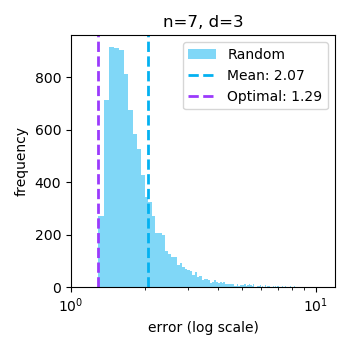
At this point I have gotten lazy and find this matrix by alternating 1) Gram-Schmidt to orthonormalize the columns and 2) rescaling the norms of the rows until convergence. Please let me know if you have an explicit initialization! I only have one via truncating/scaling Hadamard matrices which works for $n = 2^k$. This process empirically meets our criteria, showing its possible to achieve our lower bound. Putting this all together, our choice of inputs $X$ gives error $\sigma^2\frac{n^2}{d}$, which outperforms random guessing. Thank god our hard work paid off!
Though this fully solves selecting $X$ to best estimate $w$ under quadratic loss, what if we wanted to estimate $w^{\top} x_{\text{query}}$ under quadratic loss? Now, the variance contributed by each coordinate depends on the value of $x_{\text{query}, i}$ for a new objective of minimizing $\sum_{i\in[d]} \frac{x_{\text{query}, i}^2}{\lambda_i}$. This is solved when $\lambda_i = \left\{\frac{nx_{\text{query}, i}^2}{\|x_{\text{query}}\|_2^2}\right\}_{i\in[n]}$, leading to different optimal inputs.
Application to Scaling Laws
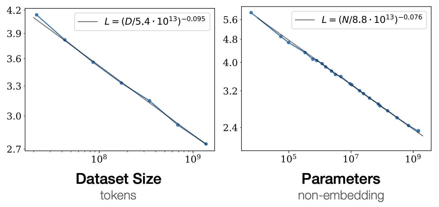
One currently prominent example of linear regression is scaling laws. It has been observed that for training language models, log error (perplexity) is linearly determined by log compute (where compute is roughly number of parameters times number of tokens) (Kaplan et al, 2020). Engineers will train $n$ models of varying scale to fit this line, which can be used to predict the performance of a model at a higher compute level. These lines are typically fit with points equally spaced out along the $x$-axis (exampled in Figure 2). Is this the optimal way to determine slope? In the following, we will consider a toy problem inspired by this problem setting. It is worth reiterating that the following math is more a fun application of our design tools rather than a reccomendation for practitioners. Regardless, the following results are surprising (to me), even from a purely mathematical perspective.
Suppose we were allowed to pick $c_i \in \R$, corresponding to the log compute spent on training model $i \in[n]$. Then, if we had to fit the model $w_1 + w_2 c_{\text{query}}$, we can solve a regression problem with inputs $X \in \R^{n\times 2}$ where the first column is all $1$'s and the $i$th row of the second column is the log compute $c_i$'s. If this is the case, assuming the same noise model as earlier, we find that the covariance matrix is
\[ \begin{aligned} & \text{Cov}(w) \\ &= \sigma^2(X^{\top}X)^{-1} & \text{[derived earlier]} \\ &= \sigma^2\begin{bmatrix} n & \sumc \\ \sumc & \sumsqc \end{bmatrix}^{-1} & \text{[explicit $X$]} \\ &= \sigma^2 \frac{1}{n\sumsqc - \p{\sumc}^ 2} \begin{bmatrix} \sumsqc & -\sumc \\ -\sumc & n \end{bmatrix} & \text{[invert matrix]} \\ \end{aligned} \]
which means the variance of the intercept is $\frac{\sigma^2\sumsqc}{n\sumsqc - \p{\sumc}^ 2}$ and the variance of the slope is $\frac{\sigma^2n}{n\sumsqc - \p{\sumc}^ 2}$. In the following, we will ignore the constant factor of $\sigma^2$.
Upper Bound Budget
We'll now start determining the optimal inputs under different constraints. First, consider a fixed number of runs $n$. To minimize the variance of the intercept, it is best to select arbitrarily smaller runs, under which the variance approaches $\frac{\sigma^2}{n}$. To minimize the variance of the slope, we have to maximize the denominator, which is proportional the sample variance of $c$. Since we could arbitrarily increase this by sending one log compute $c_i \to \infty$, we'll instead bound the values by budget $B$. In this case, the sample variance is maximized by putting half the points at $0$ and half the points at the budget $B$ (since this sets the mean to $\frac{B}{2}$ while each point has maximal distance to the mean).
Linearly Constrained Budget
For a more realistic compute constraint, what if we have a total budget with a linear constraint of $\sumc = B$? Note that this is not perfect since $c_i$ is log compute, not compute. For fixed $n$ and $B$, for both the intercept and slope, we now need to maximize $\sumsqc$ subject to the sum constraint. By simple convexity arguments, this is maximized by setting all of the runs to minimal log compute except for one run that receives $B$ log compute. After this, more runs $n$ (i.e. adding more zero runs) will decrease the variance of both the slope and intercept. Therefore, it is best to allocate one run to the full compute with as many small runs as possible.
Exponentially Constrained Budget
The most realistic constraint is that the amount of compute is fixed, captured by $\sumec = B$. We will introduce dummy variables that measure compute $d_i = e^{c_i}$, equivalently written $c_i = \log d_i$, making the constraint linear in compute $d_i$ with the additional constraints that $d_i \geq 1$. We will focus on minimizing the variance of the slope, which is now maximizing the sample variance of $\log d_i$.
One might hope that for a fixed number of runs $n$, the optimal solution scales with budget $B$ like our last two constraints. We are not this fortunate: though the denominator does not change if we linearly scale compute $d$, $d_i \geq 1$ prevents us from arbitrarily scaling down. I have lost a bit of steam here, and have empirically found with Gurobi that the optimal solution is always $d_{1}, \ldots, d_{n-k} = 1$ and $d_{n-k+1}, \ldots, d_{n} = \frac{B - n + k}{k}$ for some $k$ which interestingly depends on the choice of $B, n$. For a choice of number of big runs $k$, we find that the denominator is $(nk - k^2)(\log (B - n + k) - \log k)$. At small budgets $B$, it is unclear which $k$ is best and can be found numerically (exampled in Table 1). We empirically find that as we send $B \to \infty$, the optimal number of big runs $k$ scales like $\frac{n}{2}$, which means that the optimal solution is to evenly divide the runs between $d_i = 1$ and $d_i = \frac{2B}{n} - 1$. This qualitatively shows that the exponential constraint behaves more like the fixed upper bound regime instead of the linear constraint regime.
$B$ |
$10.5$ |
$12$ |
$24$ |
$48$ |
$480$ |
$1200$ |
$4800$ |
Best $k$ |
$1$ |
$2$ |
$3$ |
$4$ |
$4$ |
$5$ |
$5$ |
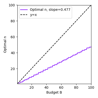
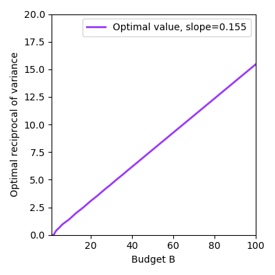
How do we select the optimal $n$? We simulate all possible choices of runs $n$ and big runs $k$ and see what works best at different budgets, shown in Figure 3. We surprisingly find a clean law of setting $n \approx 0.477B$ (left). The reciprocal of the variance of the slope magically follows a straight line as well (right), which means that the variance is inversely proportional to the budget. The second line is not surprising conditioned on the first line: if it is optimal to set $n = 0.477 B$ and $k = \frac{n}{2}$, then the reciprocal of the variance of the slope is linear with respect to $B$ with slope $0.138$. I guess that's kind of close to the empirical fit of $0.155$! However, I do not have such an explanation for why the left plot follows a line.
If we wanted to minimize the variance of estimating the error for a model of size $T$, we would want to minimize $\text{Var}(w_1) + T^2 \text{Var}(w_2)$. Though we do not consider this problem here, it can be solved using simple programs like above. Its worth noting that as we increase $T$, the variance of the slope dominates the intercept, even if we correspondingly scale $B$.
Parting Thoughts
Under a simple noise model, we've shown how to optimally select inputs, which significantly outperforms random sampling. We took this to a scaling law problem where the optimal input selection was counter-intuitive (at least to me). Most surprising to me is that it never made sense to space out the inputs: it was always best to keep all at the minimum or maximum. There are obviously other reasons to equally space out points, such as confirming the law is linear in the first place. Nonetheless, I'm curious which settings lead to spacing out points being optimal. There are some natural followups such as modeling the fact that noise is lower for more compute (shown in Jordan et al, 2023).
Deriving these simple results from first principles was a blast. I hope to run into this flavor of problems someday if I start running large-scale experiments. Thanks to Ankit Bisain, Jacob Springer, and Mahbod Majid for tolerating my yapping and helping me with some math.
Thank you for reading, and feel free to reach out with any questions or thoughts!