Paper Analysis: Provable Guarantees for Self-Supervised Deep Learning with Spectral Contrastive Loss
\( \def\truedist{{\overline{X}}} \def\allset{{\mathcal{X}}} \def\truesample{{\overline{x}}} \def\augdist{\mathcal{A}} \def\R{\mathbb{R}} \def\normadj{\overline{A}} \def\pca{F^*} \def\bold#1{{\bf #1}} \newcommand{\Pof}[1]{\mathbb{P}\left[{#1}\right]} \newcommand{\Eof}[1]{\mathbb{E}\left[{#1}\right]} \)9/28/2023
Given a lot of unlabelled data and a little labelled data, our best method of leveraging it is probably contrastive learning. Though we can intuitively explain why it works, its difficult to truly explain its power. The brilliant work of HaoChen et al, 2021 explains how contrastive learning can be explained as implicit spectral clustering. Along the way, they show how to use this insight to improve practice! The original paper has a genuinely beautiful exposition so please defer to them for the full math, setup, and details. This post will serve as a shorter and simplified introduction, touching on some necessary background, aspects I personally find interesting, and further contextualization with respect to the field.
Background
The goal of contrastive learning is to convert inputs without labels into embeddings \(\R^k\) such that similar images have close embeddings and dissimilar images have far embeddings. These embeddings give some "general understanding" of the data distribution, which can be efficiently adapted to downstream tasks (e.g. classification, clustering, similarity search) with little to no data.
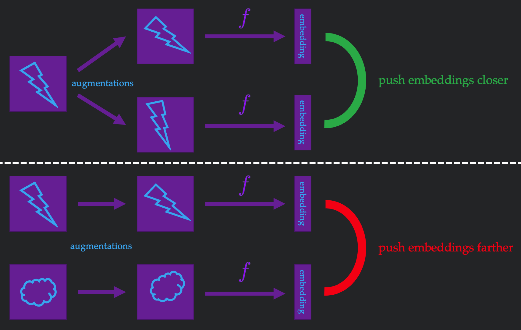
Since the images have no labels, it seems pretty hopeless to get any understanding of our data. However, we can get some insight by considering augmentations of images (e.g. jittering the color, rotating the image, randomly cropping, etc). The key observation is that augmentations of the same image should be quite similar, and augmentations of different images should be quite different. Therefore, if we were learning an embedding function \(f\), we could measure whether our embeddings satisfy this property for augmentations of the same image and augmentations of a random pair of images, as stylized in Figure 1. Every time we play this little game, we can keep adjusting our \(f\), which intuitively makes our embeddings better and better.
This algorithm approach, best represented by SimCLR (Chen et al, 2020) is one of the best methods we currently have for image classification. Today, we will theoretically explain why it works!
Setting
We'll consider the "true" data distribution as \(\truedist\) and draw samples \(\truesample \sim \truedist\). To run self-supervised learning, we need to be able to augment the image in a way that preserves similarity. We'll define an augmentation via its distribution given an input sample. More precisely, the likelihood of a point \(\truesample'\) coming from \(\truesample\) is given by the likelihood \(\augdist(\truesample' \mid \truesample)\). Given this augmentation distribution, our goal will be to find an embedding function \(f : \allset \to \R^k\) that produces "good embeddings" of dimension \(k\) for any valid image \(x \in \allset\). Good embeddings can mean different things for different downstream tasks, so we consider the concrete task of training a linear classifier over \(r\) classes. Combining all these components, our optimization problem boils down to
\[\min_{f} \min_{B \in \R^{k\times r}} \mathbb{P}_{\truesample \sim \truedist}\left[Bf(\truesample)\text{ misclassifies }\truesample\right]\]
Population Graph
To begin finding embeddings, we need to consider what information we want our embeddings to preserve. A natural idea is for the embeddings to capture similarity between images. How do we define similarity without labels? The only "supervision" we have in this case is that our provided augmentation preserves similarity. Therefore, if two images are likely to be generated from the same augmentation, we could considered them similar, and the inverse as well. We can operationalize this intuition by making an similarity matrix \(A\) where each entry is \[w_{x_1x_2} := \mathbb{E}_{\truesample \sim \truedist} \left[\augdist(x_1 \mid \truesample) \augdist(x_2 \mid \truesample)\right]\] This matrix, which has a row and column for every possible image from the set \(\allset\), can tell us how similar \(x_1\) and \(x_2\) are. Note that the set \(\allset\) of \(N\) possible images is not the same as the support of \(\truedist\), since augmentations can create images that might not exist in nature. Since some images may just naturally be more similar to every image, we can further normalize this to produce matrix \(\normadj\) where each entry is scaled down by \(\sqrt{w_{x_1}w_{x_2}}\) for row sum \(w_x = \sum_{x'\in \allset} w_{xx'} = \sum_{x'\in \allset} w_{x'x}\).
Example of Population Graph
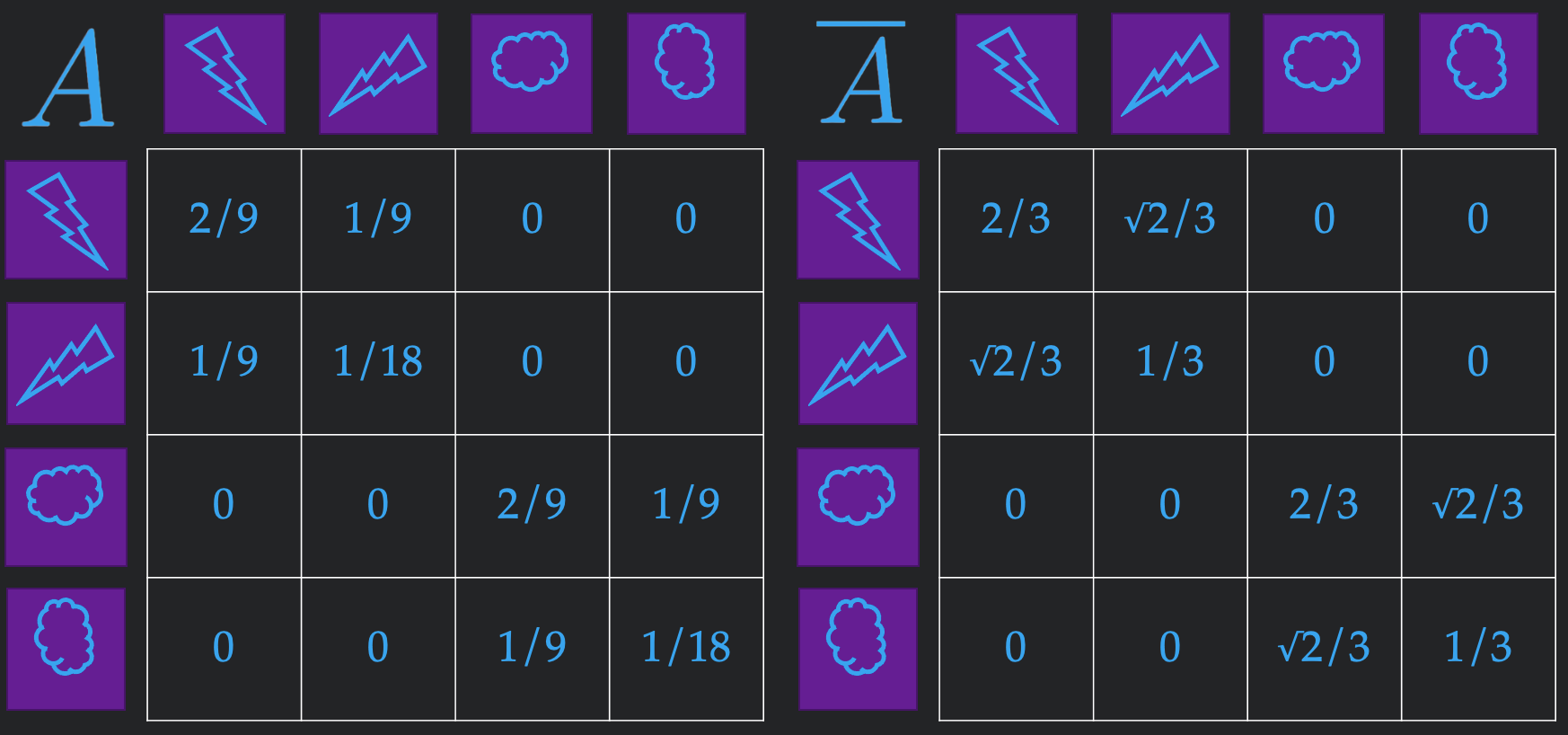
To make everything concrete, let's consider a small reasonable example. We will have two images (a lightning bolt and a cloud) in the support of our \(\truedist\) with equal likelihood. For our augmentation, we will consider vertically rotating the image with probability \(\frac13\), and otherwise keeping it the same, described by the augmentation distribution
\[\augdist(\cdot \mid x) = \begin{cases}\text{Rotate}(x) & \text{with probability } \frac13 \\ x & \text{with probability } \frac23\end{cases}\]
With this, we can construct our similarity matrix as shown in Figure 2 (justify to yourself the values in each entry using our earlier definitions). We first observe that even though our true distribution \(\truedist\) only had two images, our population graph has 4 possible images, since the augmentations increase the space of feasible images. We also notice that when looking at this as a graph, similar images naturally cluster, making it a suitable representation for downstream tasks.
Using the Population Graph
It seems like this matrix could contain all the information one could ever dream of. How can we derive \(k\)-dimensional embeddings? If our matrix is of dimension \(N\times N\), we can consider each row of our matrix \(\normadj\) as an \(N\)-dimensional embedding of an input. We can perform Principal Component Analysis (PCA) to keep the top \(k\) eigenvectors of the matrix, producing the matrix \(\pca \in \R^{N\times k}\) pictured in the following diagram. The \(i\)th column of \(\pca\) corresponds to eigenvector \(v_i\), and the \(j\)th row of this matrix corresponds to a \(k\)-dimensional embedding of image \(j\). This corresponds to the notion of Spectral Clustering, or using the spectrum of the adjacency matrix to cluster images. We know that PCA provides the provably optimal low-rank approximation of a matrix, so in some sense, this is the best method of preserving as much information as possible in our \(k\)-dimensional embeddings!
\[ \underbrace{\begin{bmatrix} & \vdots & \\ & \vdots & \\ \ldots\ldots & \frac{w_{x_1x_2}}{\sqrt{w_{x_1}w_{x_2}}} & \ldots \ldots \\ & \vdots & \\ & \vdots & \end{bmatrix}}_{\normadj \in \R^{N\times N}} \quad \underbrace{\Longrightarrow}_{\text{PCA}} \quad \underbrace{\begin{bmatrix} \bigg| & \bigg| & \bigg| \\ & \phantom{\vdots} & \\ v_1 & \ldots & v_k \\ & \phantom{\vdots} & \\ \bigg| & \bigg| & \bigg| \end{bmatrix}}_{\pca \in \R^{N\times k}}\]
In practice, augmentations can generate many variations of an image, and this \(N \times N\) matrix is basically \(\infty \times \infty\)!!! We can not compute, store, or leverage this matrix in any manner, and at first glance it seems pretty doomed to get anything useful out of this. However, fret not, because machine learning comes to the rescue!
Learning the Population Graph
Is there any hope of finding \(\pca\)? Even the PCA representation has an infinite number of rows! Well, this matrix corresponds to a table of every possible embedding. As computer scientists, our gut reaction is to refactor this as a function that outputs an embedding given an input, rather than explicitly storing this mess. In fact, this \(f\) an embedding function for any possible input, which is exactly what we've been looking for! This \(f\) only has to produce matrix \(F\) that's within an invertible linear transformation of \(F^*\), since our linear classifier \(B\) on top can undo any effects as necessary. For (at the moment) magical reasons, we will try to find an \(f\) such that the embedding of \(x\) is approximately \(w_x^{1/2}f(x)\), as depicted below.
\[ \underbrace{\begin{bmatrix} \bigg| & \bigg| & \bigg| \\ & \phantom{\vdots} & \\ v_1 & \ldots & v_k \\ & \phantom{\vdots} & \\ \bigg| & \bigg| & \bigg| \end{bmatrix}}_{\pca \in \R^{N\times k}} \quad \underbrace{\approx}_{\text{the dream}} \quad \underbrace{\begin{bmatrix} \phantom{\bigg|} & \vdots & \\ & \phantom{\vdots} & \\ - & w_x^{1/2}f(x) & - \\ & \phantom{\vdots} & \\ & \vdots & \end{bmatrix}}_{F \in \R^{N\times k}} \]
It is incredibly non-obvious how we are going to find such an \(f\). But lets don our optimism hat, and work through quantifying the gap between \(\normadj\) and \(F\) for a chosen \(f\).
\begin{aligned} & \min_{F\in \R^{n\times k}} \|\normadj - FF^{\top}\|_F^2 & \text{[low-rank approx]}\\ &= \min_{f : \allset \to \R^k} \sum_{x_1, x_2 \in \allset} \left(\frac{w_{x_1x_2}}{\sqrt{w_{x_1}w_{x_2}}} - (w_{x_1}^{1/2}f(x_1))^{\top}(w_{x_2}^{1/2}f(x_2))\right)^2 & \text{[Frobenius norm]}\\ &= \min_{f : \allset \to \R^k} \sum_{x_1, x_2 \in \allset} \frac{w_{x_1x_2}^2}{w_{x_1}w_{x_2}} - 2w_{x_1x_2}f(x_1)^{\top}f(x_2) + w_{x_1}w_{x_2} \left(f(x_1)^{\top}f(x_2)\right) & \text{[expand terms]}\\ &= \min_{f : \allset \to \R^k} \sum_{x_1, x_2 \in \allset} - 2w_{x_1x_2}f(x_1)^{\top}f(x_2) + \sum_{x_1, x_2 \in \allset} w_{x_1}w_{x_2} \left(f(x_1)^{\top}f(x_2)\right) & \text{[remove constant]}\\ &= \min_{f : \allset \to \R^k} - 2 \mathbb{E}_{x_1, x_2 \sim \augdist(\cdot \mid x \sim \truedist)}\left[f(x_1)^{\top}f(x_2)\right] + \mathbb{E}_{x_1 \sim \augdist(\cdot \mid x \sim \truedist), x_2 \sim \augdist(\cdot \mid x \sim \truedist)}\left[f(x_1)^{\top}f(x_2)\right] & \text{[rewrite sum]}\\ \end{aligned}
where \(\sim\augdist(\cdot \mid x \sim \truedist)\) is an abuse of notation for sampling an augmentation \(\augdist\) from a sample of the true distribution \(\truedist\). What does all of this fun algebra say? Well, let's take a look at the expectation that pops out at the bottom. It's important to note that though the distribution we're sampling over looks similar in both expectations, they are not to be confused with each other. We can analyze the decomposition for an English interpretation.
\[- 2 \underbrace{\mathbb{E}_{x_1, x_2 \sim \augdist(\cdot \mid x \sim \truedist)}\left[f(x_1)^{\top}f(x_2)\right]}_{\substack{\text{embeddings agreement on} \\ \text{augmentations of the same image}}} + \underbrace{\mathbb{E}_{x_1 \sim \augdist(\cdot \mid x \sim \truedist), x_2 \sim \augdist(\cdot \mid x \sim \truedist)}\left[f(x_1)^{\top}f(x_2)\right]}_{\substack{\text{embeddings agreement on} \\ \text{a pair of random images}}}\]
- The first expectation samples two augmentations of the same image, which means that most likely, the two images are related. Minimizing the negative expectation makes the dot product of the "related" embeddings larger, pushing them closer to each other.
- The second expectation samples two images randomly, which means that most likely, the two images are unrelated. Minimizing the expectation makes the dot product of the "unrelated" embeddings smaller, pushing them further away from each other.
Putting this all together, the above expectation captures how desirable our embedding function is. Now we can sample this loss function through augmenting our images. This gives us an approximation of the loss we can differentiate through with respect to the parameters of \(f\). Therefore, we can use the standard ML toolkit of taking a huge neural network, seeing the loss, and taking a gradient step in a direction that minimizes the loss! As we continue to optimize this loss function, we continually improve the quality of our embeddings, which leads to better and better downstream performance.
Interestingly, this loss function resembles the loss function used by practitioners such as the InfoNCE loss of SimCLR, where similar images are pushed closer together and random images are pushed further away from each other. Therefore, this analysis sheds some insight into why self-supervised learning works so well in practice!
Theoretical Generalization
In essence, the paper leverages the following assumptions.
- The adjacency matrix \(A\) naturally forms a few tight clusters
- Unlike prior work (Arora et al, 2019), they do not require that each class is exactly one cluster
- The formal criterion relies on the conductance of a graph which is important quantity to spectral graph theory, refer to Definitions 3.3-3.4 and Assumption 3.5 of the paper if interested.
- Augmentations preserve labels with high probability
- Our class of neural networks can express the optimum to the loss function defined above
- We have a lot of unlabelled data (polynomial in problem parameters) and some linear data (linear in the representation dimension)
With these assumptions, we can prove that we produce great embeddings with great downstream classification accuracy under a linear probe. Though this may seem like a lot of assumptions, many of them are reasonable, and they paint a picture that as long as one has a good augmentation and the data is amenable to clustering, then scaling self-supervised learning will converge to spectral clustering under this similarity metric.
Empirical Generalization
It's important to note that even though this loss function resembles the loss function in practice, its slightly different. What's amazing is that using this more theoretically principled function makes self-supervised learning easier! Though this paper doesn't push numbers significantly past the state of the art, they find that this new loss allows them to drop a lot of previous heuristics such as large batch sizes, momentum encoders, and stop-gradient methods. This is really exciting since it shows that the mathematical analysis offers value to the immensely useful practice of self-supervised learning!
What's left to understand here? (My thoughts)
This phenomenal paper provides a compelling explanation of self-supervised learning, almost making it feel simple. Here are my thoughts on some interesting directions following this paper, some of which have been subsequently explored, and others which will require some brave researchers to solve :))
Difference between contrastive learning and self-training
Self-training (a form of semi-supervised learning) offers another method of leveraging unlabelled data for improved downstream performance. The beautiful work of Shen et al, 2021 shows how self-training under similar assumptions leads to similar generalization guarantees. In fact, both papers share similar theoretical guarantees for performance under a mixture of manifolds. Aditi posed to me the wonderful puzzle of determining when self-supervised learning is better than self-training or vice versa. I do not have a great understanding of when they differ, but some recent work might!
Inductive Biases
Suanshi et al, 2022 take a careful look at the assumptions given through this spectral analysis, and rezognize that these bounds can not leverage inductive biases present in the network architecture and training algorithm. They find that simply varying the function class or optimizer across various domains causes large shifts in performance, even though the spectral analysis should not change for a static augmentation and data distribution. Therefore, though the spectral bounds are true, they do not completely explain performance in practice, and there is more work to be done in leveraging inductive bias. The follow-up work HaoChen et al, 2023 offers a more nuanced analysis of contrastive learning by leveraging inductive biases of function classes. However, it is worth noting that we are very far from understanding the inductive biases of optimization and neural networks in general, and a lot more research is necessary for tight claims.
Understanding the Projection MLP
This work manages to remove a lot of tricks, though they still require the trick of using a two layer neural network as the classification head rather than a linear layer. This is fine for practice, but raises an interesting question of where the theoretical analysis is incongruent with the practical implementation. This might provide further insight into the embedding space that is not captured by the analysis in this paper.
Summary
Optimizing a simple contrastive loss function can be equivalent to implicitly spectrally clustering the data, which offers great downstream performance for many data distributions. This offers strong insight into why the practice of constrastive learning has been so successful!
Thank you for reading, and feel free to reach out with any questions or thoughts!