Down to the basics
The camera
The exact camera used by Prokudin-Gorsky remains unknown, but it is believed to have been similar to the Miethe-Bermpohl three-color camera, as shown below. Descriptions suggest his camera was a compact, wooden folding model equipped with a repeating back. The negatives, long glass plates measuring 9 x 24 cm, are a testament to the unique photographic process he employed.
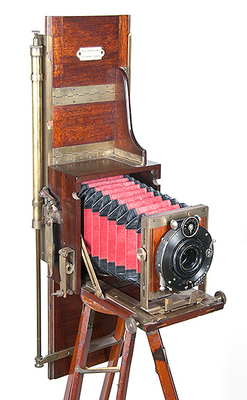
Three-Color Camera
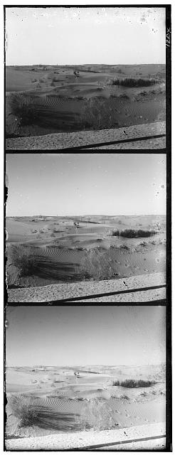
Glass Negative
Sufficiency of Basic Transitions
In contrast to film, which can warp and deform, glass plates maintain their rigidity, thus preserving the alignment of the three color channels. My experiments demonstrate that employing transitions along these axes alone is sufficient for achieving high-quality alignment, with more complex techniques offering only marginal improvements.
Color accuracy
Prokudin-Gorskii used 3 filters to capture the three color channels. It's likely that his color filters are not perfect, thus projecting the color channels directly to the RGB space will not be accurate. The sensitivity of the the negative is also not uniform, and since he took each channel separately, the exposure time for each channel is different. All these factors could contribute to the inaccuracy of the color channels, and this is a subject that yet to be explored.
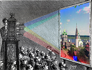
Triple-Color Projection. Illustration by Dr. Victor Minachin
Single-scale & Pyramidal Alignment
I initially developed the single scale function and subsequently integrated the pyramidal structure by leveraging this function. While the pyramidal search effectively reduces the search space, it's not a panacea. The 4D search process, encompassing x&y transitions as well as scale and rotation adjustments, remains computationally intensive.
To assess the alignment's effectiveness, I utilized three metrics: the sum of squared differences (SSD), the normalized cross correlation (NCC), and the zero-mean normalized cross correlation (ZNCC). Despite producing similar outcomes, the latter two metrics proved to be more time-consuming for processing large images. Therefore, I opted for the SSD metric for the final implementation.
Although the results are not flawless, they represent a significant step forward. The outcomes are detailed below.

Different Metrics
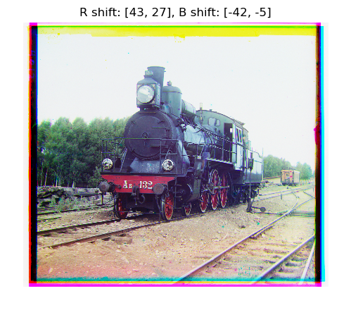

Processing time: Pyramidal(43s) vs Single-Scale(3m13s)
Improvements
Use 🌳Green channel as reference
A detailed examination of the original negatives reveals that the green channels, positioned centrally among the plates, are generally the best preserved. Conversely, the blue and red channels often exhibit damaged edges, which could lead to inaccurate alignment.
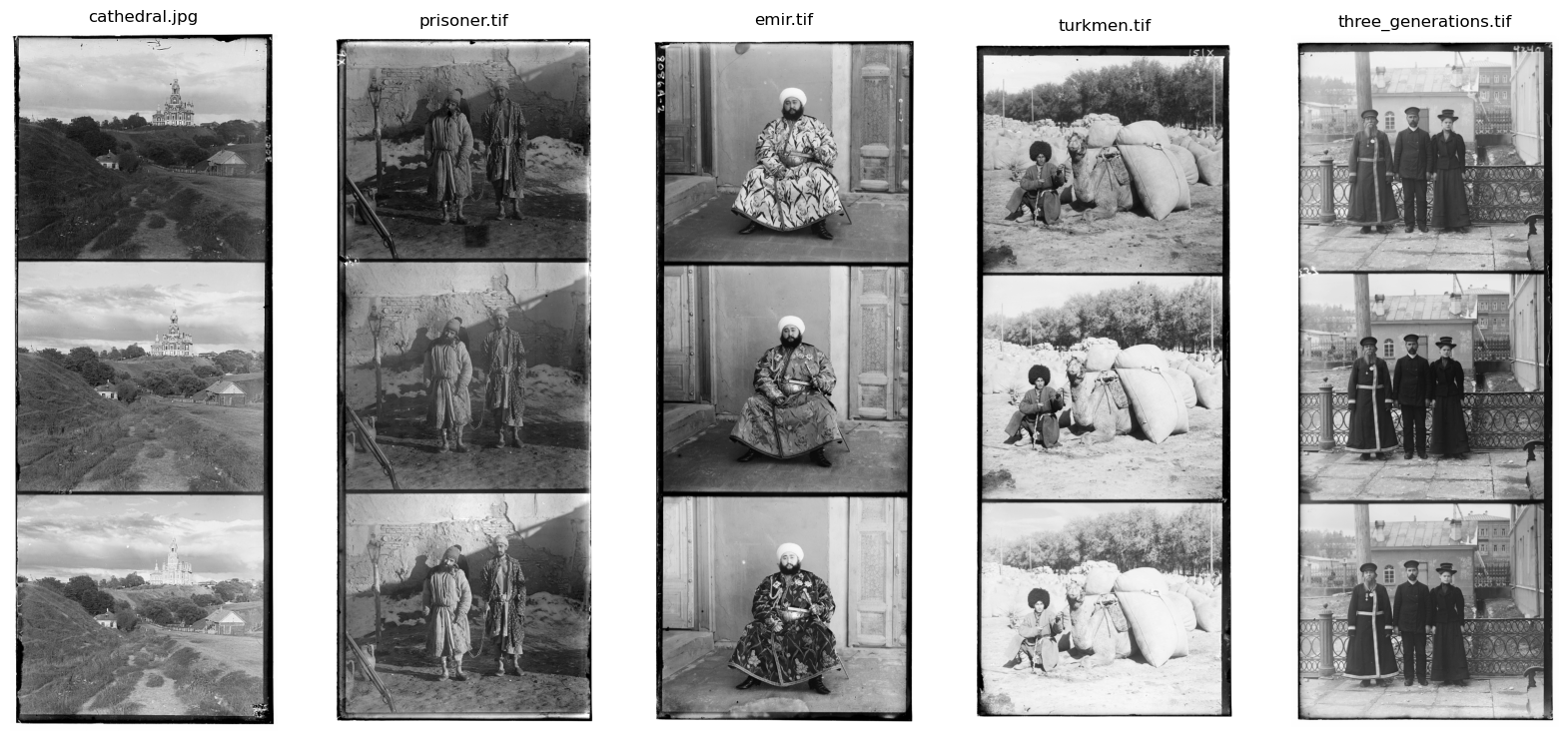
Original negatives
Below is a comparison of alignment results using the green and blue channels as references. With identical parameters, utilizing the green channel consistently yields superior outcomes.
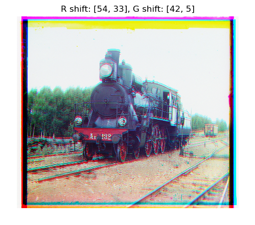

Comparison of using green and blue channel as reference
Shift Mode Matters
When shifting channels, determining how to manage the edges is crucial. This detail may seem minor, but in cases where the difference between two images is slight, the treatment of edges can significantly influence the computed metric.

SSD of different Shift Modes, lower is better
The nearest shift mode in scipy.ndimage.shift typically yields the most accurate results. However, this method can be slow for large images. As a viable alternative, I've found that the wrap mode, implemented using np.roll(), offers a good balance of speed and effectiveness.
Repeated alignment and 4D seach
While pyramidal alignment is effective for reducing the search space, it doesn’t guarantee optimal results in every scenario. For instance, situations involving significant misalignment or damage to one of the channels can lead to inaccurate initial alignments, resulting in the process potentially getting trapped in a local minimum.
Expanding the search space is a possible solution for suboptimal results, yet this approach causes the computational cost to increase quadratically. To tackle this issue more efficiently, my strategy involves conducting an initial search within a limited range, followed by cropping the image edges, and finally executing a broader search. The benefits of this method are demonstrated below.
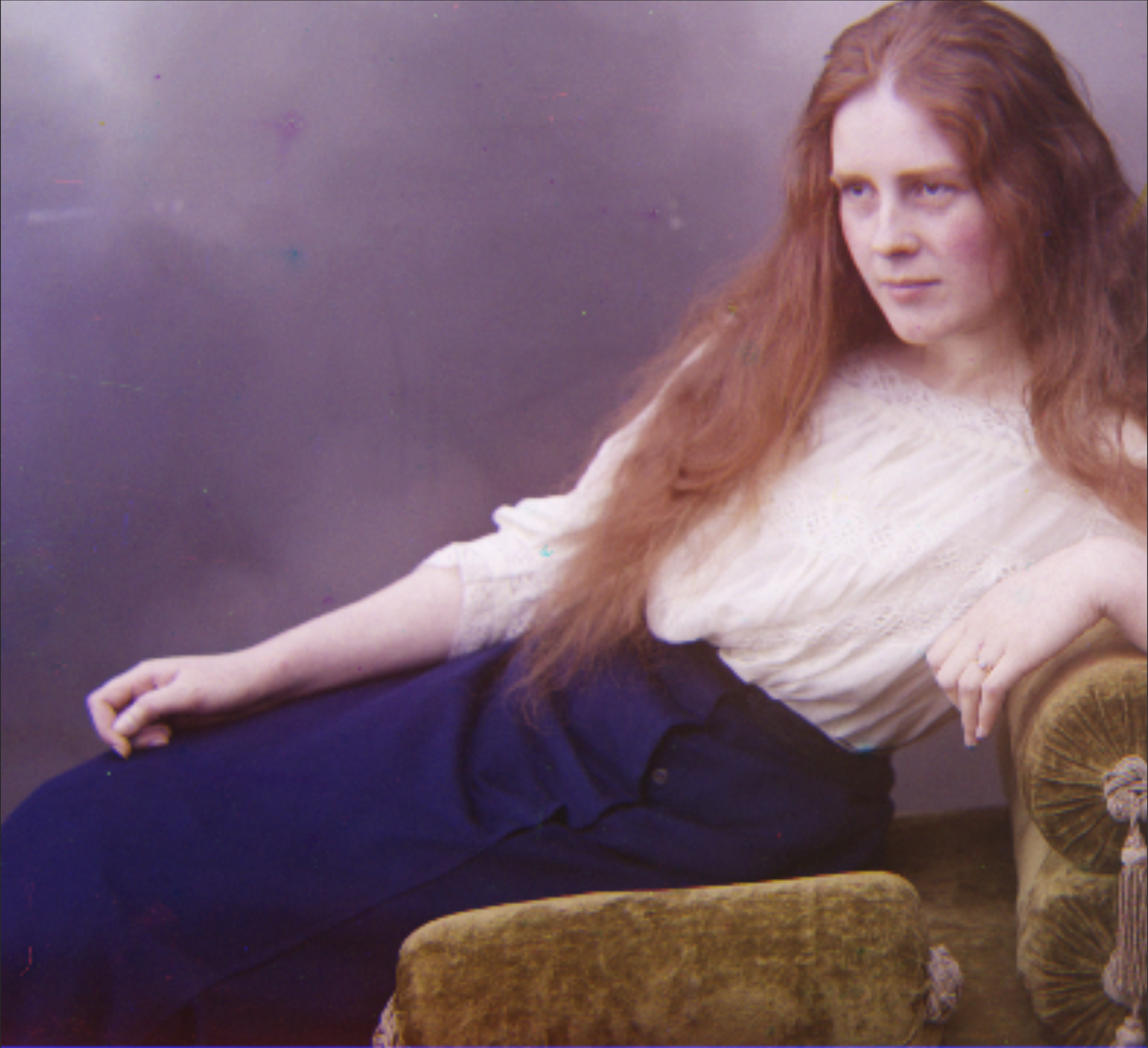
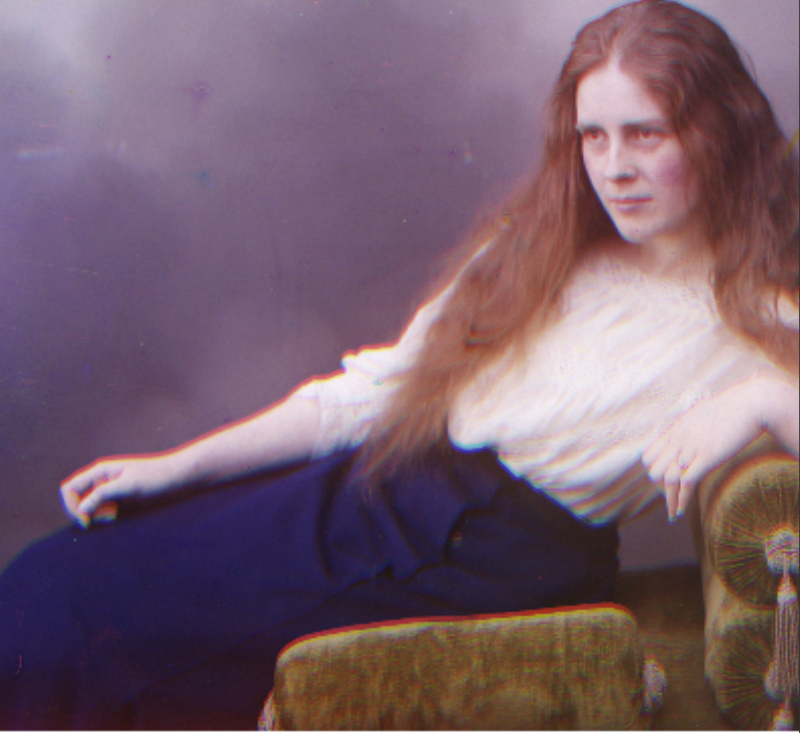
Pay attention to the difference in the hand. Enlarged for better comparison.
I experimented with a 4D search as well, but as previously mentioned, the improvements are minimal. Additionally, introducing two more dimensions makes the search more susceptible to being influenced by imperfections along the edges. The computation time significantly increases for a 4D search, taking approximately 30 minutes for a high-resolution image. This extended processing time is partly due to my use of scipy's ndimage.shift for shifting, which is less efficient than np.roll.
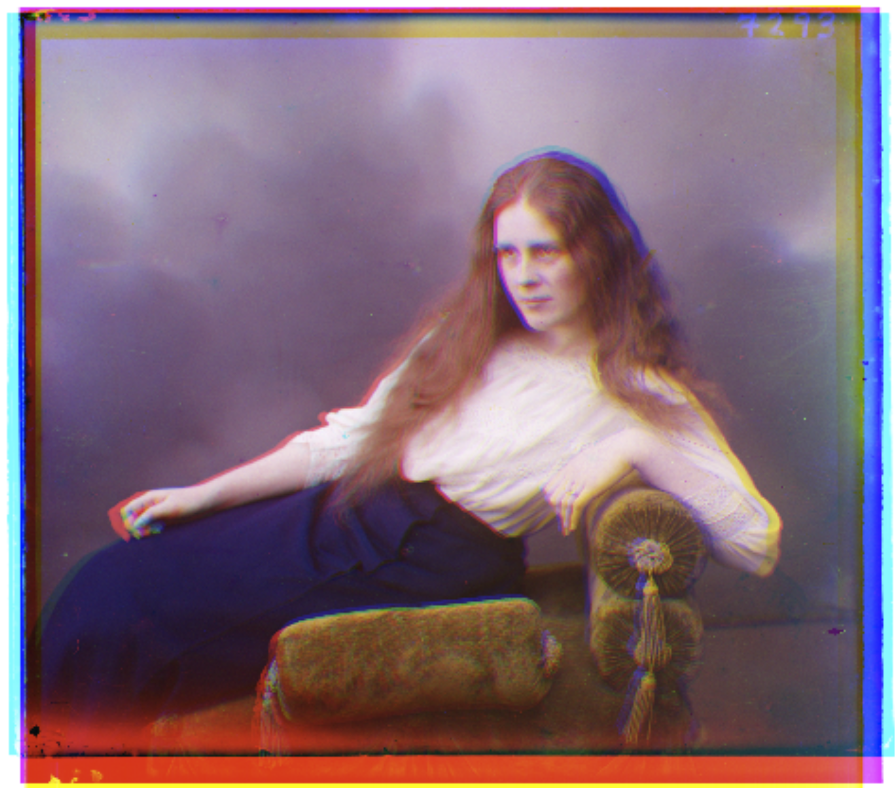
An example when 4D search yields a worse result
Better channel splitting
The traditional method of channel splitting involves dividing the image into three equal sections. However, this approach is flawed because the three channels are not distributed evenly, resulting in a loss of image parts that could otherwise be matched.
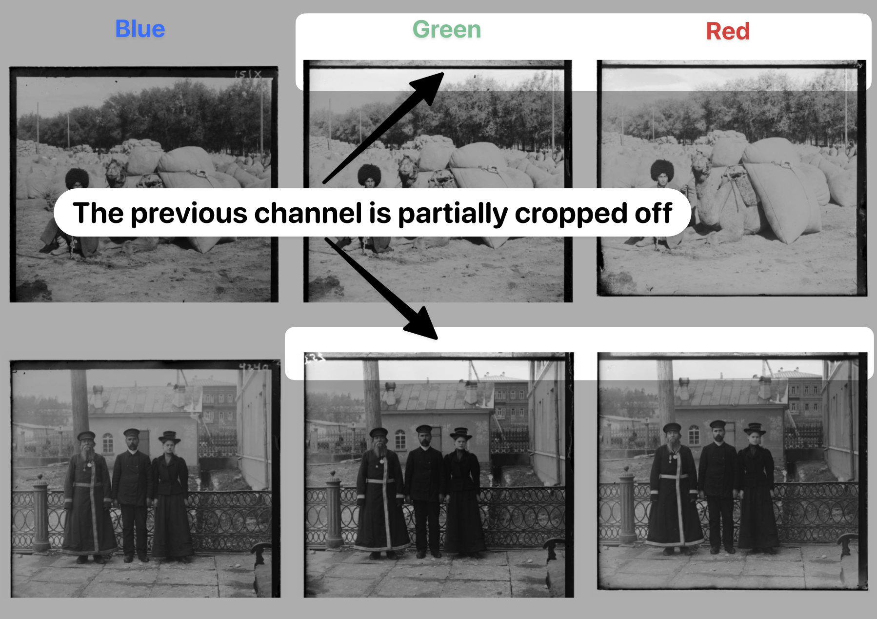
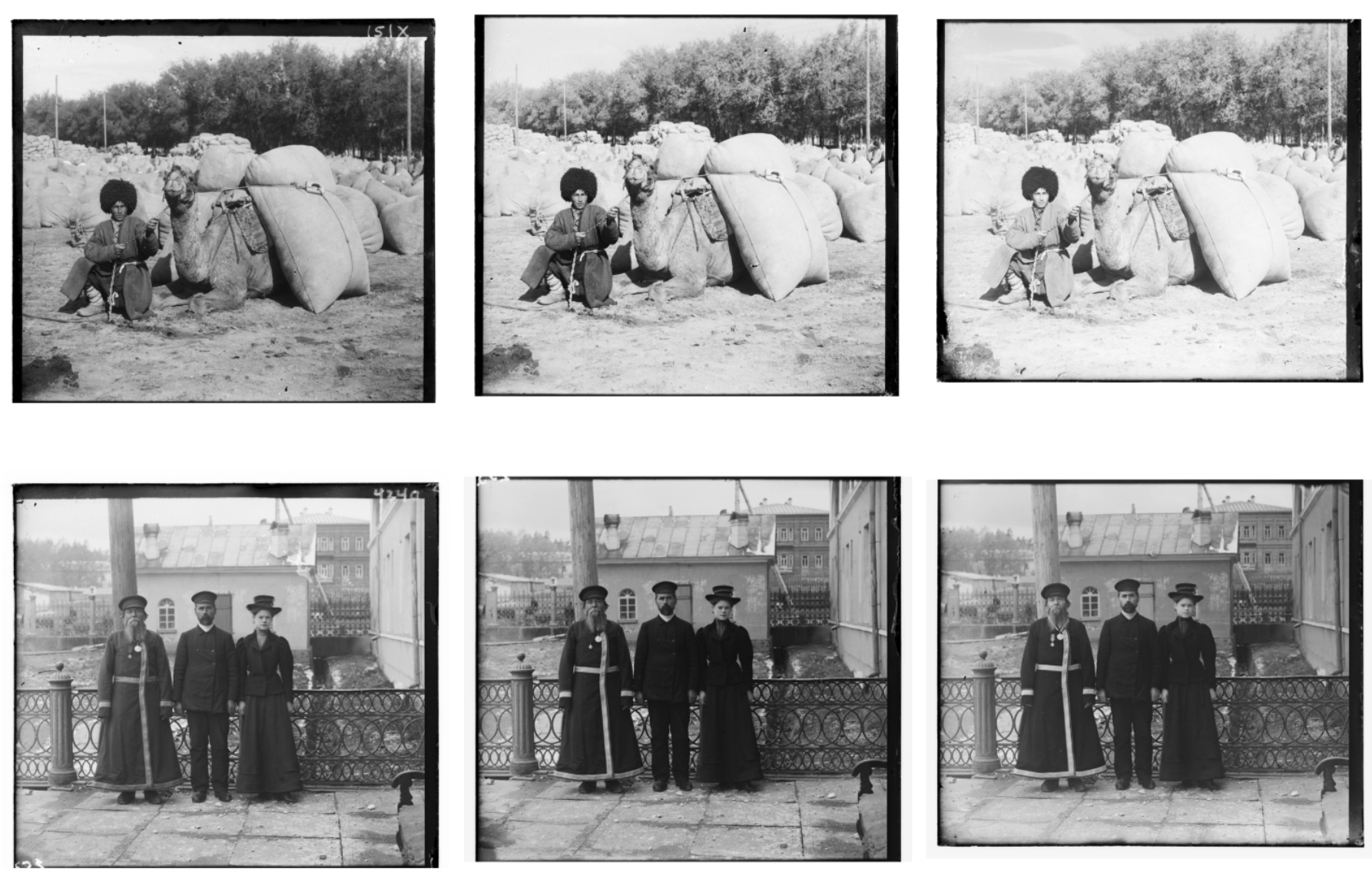
In order to split the channels more accurately, we need to automatically detect boundaries between the channels. I noticed that the boundaries is always black. Therefore, it can be simply achieved by calculating the histogram of the pixel values along axis 0 and finding the peaks.
The result is shown below.
Local wrapping using optical flow
As noted on the Library of Congress website, BGR channels are not captured simultaneously, which can result in the subject moving. Such movements can lead to ghosting effects, with common landscape elements like trees swaying, smoke from chimneys, clouds moving across the sky, and flowing water contributing to this issue. Thus, outside of carefully controlled interior still lifes, achieving perfect color alignment across an entire image is generally not feasible.
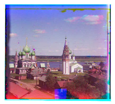
Observe the colorful cloud
To mitigate these challenges, a form of "local warping" is necessary. I employed optical flow for this purpose, a technique designed to estimate the motion of objects across successive frames. The illustration below demonstrates optical flow's capability to discern the movement of the prisoner's head.
Notice how optical flow enhances the consistency of the pattern in the prisoner's clothing and improves the alignment of the prisoner's head.
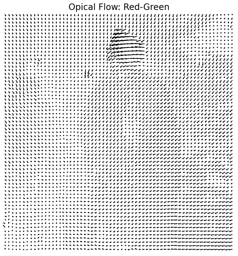
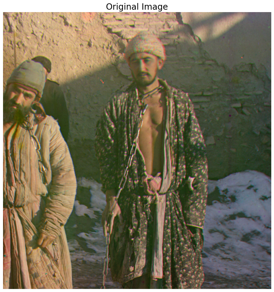
Visualizations of the optical flow

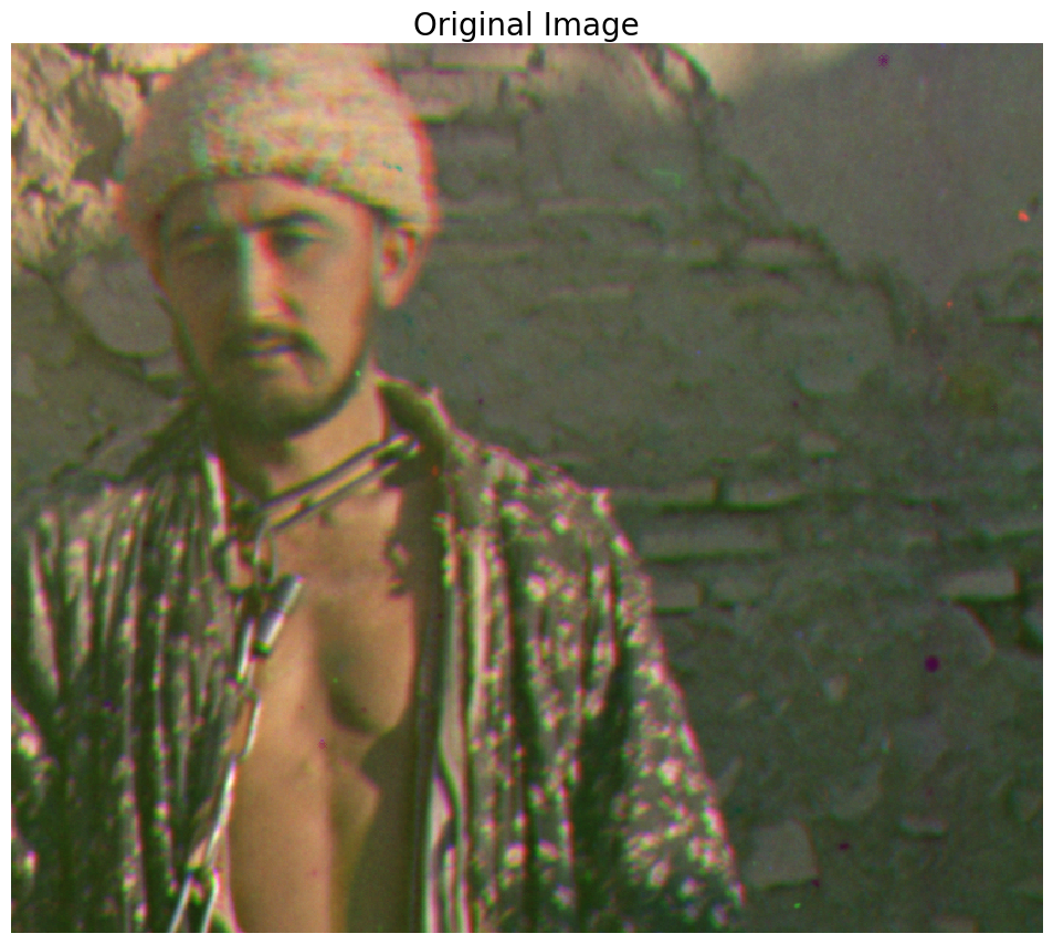
Notice the difference on the clothes, enlarged for better comparison.