Project Description
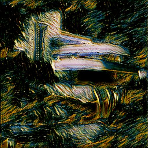
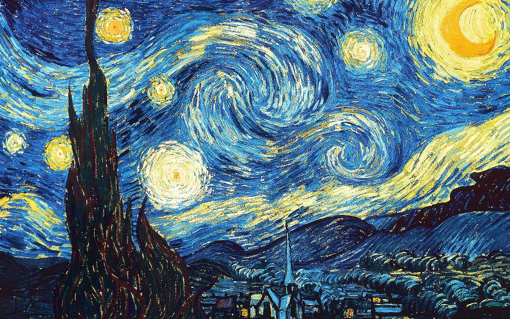
In this project, we implement the neural style transfer which resembles specific content in a certain artistic style. The algorithm takes in a content image, a style image, and another input image. The input image is optimized to match the previous two target images in content and style distance space.
We first start from random noise and optimize it in content space. It helps us understand the general idea of optimizing pixels with respect to certain losses. Then we ignore content for a while and only optimize to generate textures. This builds some intuitive connection between style-space distance and gram matrix. Lastly, we combine all of these pieces to perform neural style transfer.
I. Content Reconstruction
Content loss is a metric function that measures the content distance between two images at a certain individual layer. Here we use the squared l2-distance to measure the the distance between two features: \[ \mathcal{L}_{\text{content}, l}=|f_x^l-f_c^l|_2 ^2\] where $f_x^l$ is the $l$th-layer feature of the input $x$, and $f_c^l$ is that of the target content image $c$. We use a VGG-19 model pre-trained on ImageNet to extract features. The pre-trained VGG-19 model consists of 5 blocks (conv_1 - conv_5) and each block consists of various number of convolution layers:
- conv_1: conv_layer_1, conv_layer_2
- conv_2: conv_layer_3, conv_layer_4
- conv_3: conv_layer_5, conv_layer_6, conv_layer_7, conv_layer_8
- conv_4: conv_layer_9, conv_layer_10, conv_layer_11, conv_layer_12
- conv_5: conv_layer_13, conv_layer_14, conv_layer_15, conv_layer_16
Starting from noise map 1


Starting from noise map 2

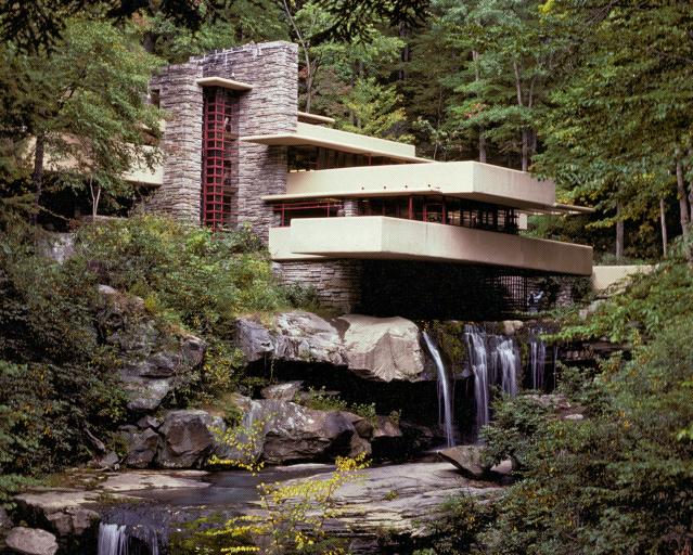
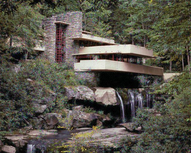

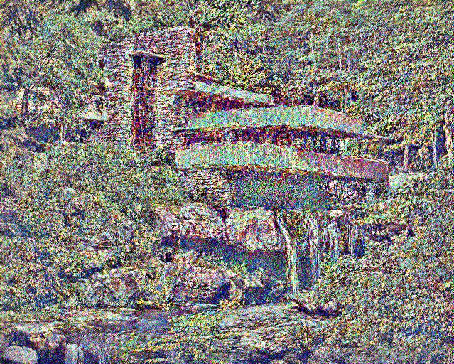

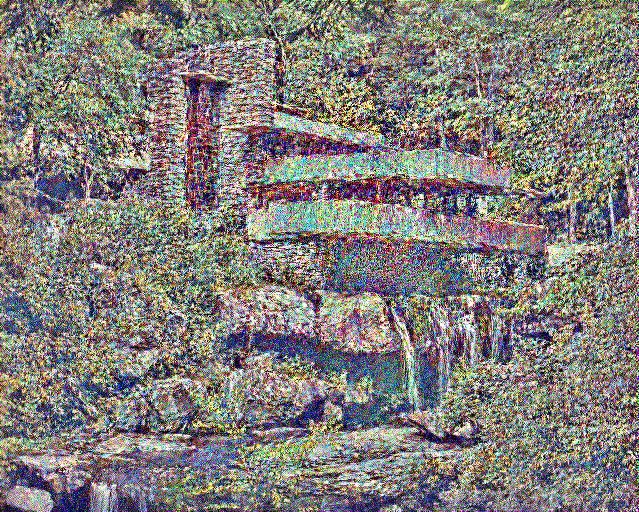
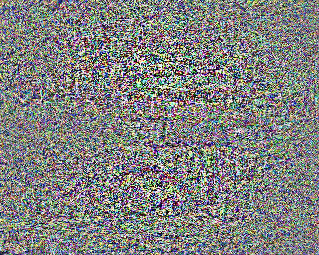
We can see that the two sets of experiments starting from different noise maps gives similar results to human eyes. The content loss on conv_1 gives the best reconstruction quality. And as the layer levels goes higher, the reconstruction quality drops. This is because the deeper layers extract higher level features that can be more abstract. Also the deeper the layer is, the smaller the feature map is, which can lead to a loss of detailed information from the original image.
II. Texture Synthesis
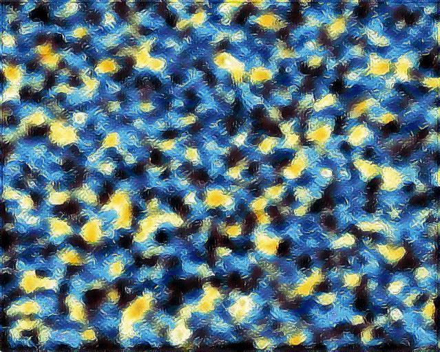
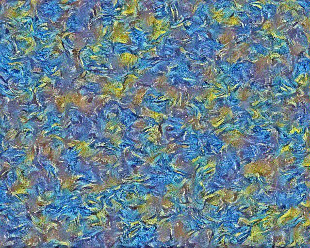
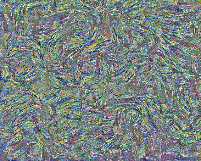
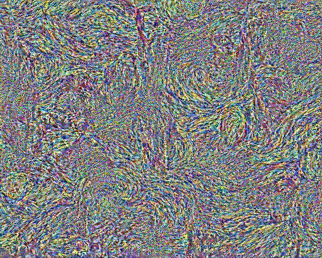
The Gram matrix is used as a style measurement. Gram matrix is the correlation of two vectors on every dimension. Specifically, denote the $k$-th dimension of the $l$th-layer feature of an image as $f_k^l$, in the shape of $(N, C, H * W)$, Then the Gram matrix is $G=f_k^l(f_k^l)^T$ in the shape of $(N, C, C)$. We again optimize the input image against the squared l2-loss between its Gram matrix and that of the target style image. And we again run the same experiment twice starting with two different noise maps. Here are the results:
Starting from noise map 1


Starting from noise map 2

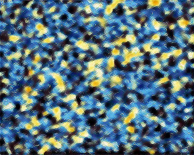

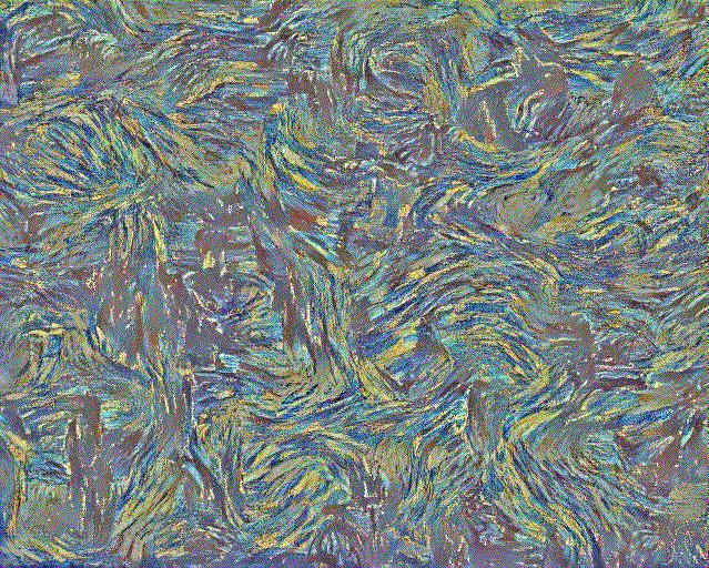
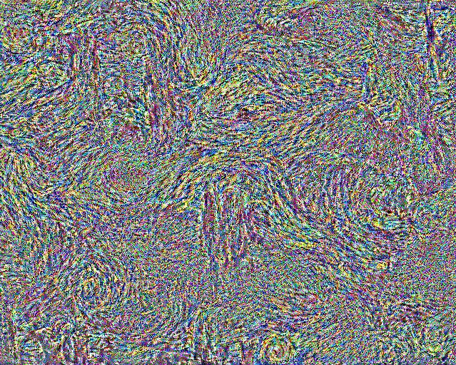

We can see that the low-level layers mainly capture the color patterns of the image, while the high-level layers capture the curves in larger scales.
III. Style Transfer
Now we can update the input image with both content loss and style loss to do style transfer. After our ablation experiments, we found that constructing the style loss with all conv_1 - conv_5 layers, and the content loss with only the conv_3 layer gives the most satisfying results. As for the loss weights, we set $\lambda_{\text{style}}=10^6$ and $\lambda_{\text{content}}=10^3$ by default. Here are the results:


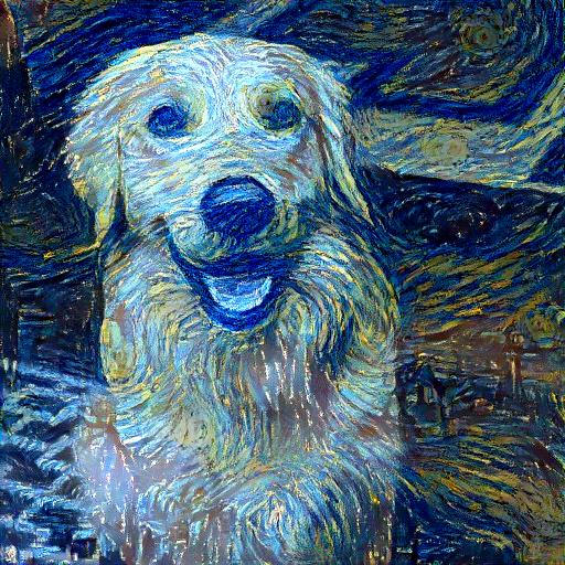
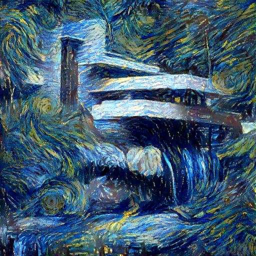
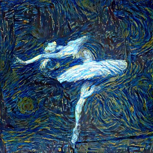
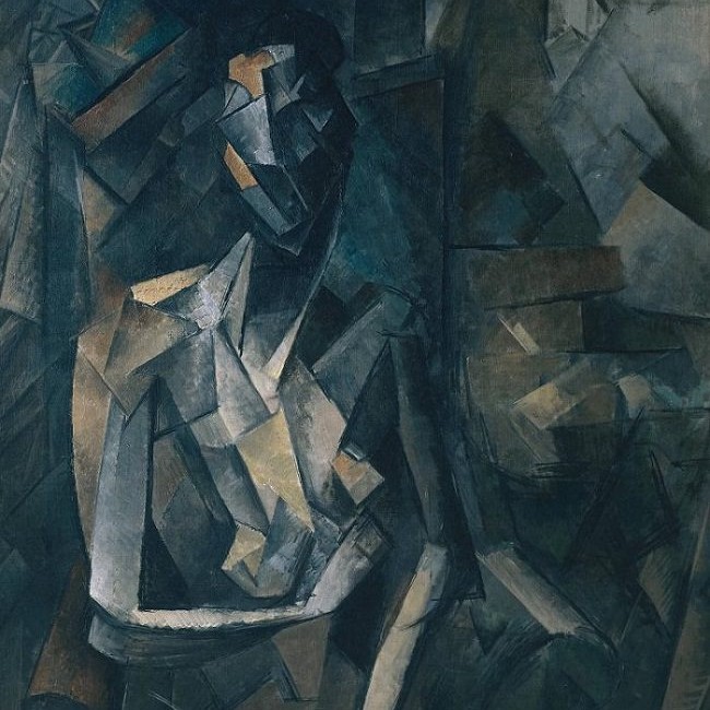
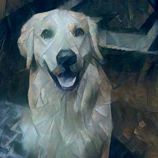
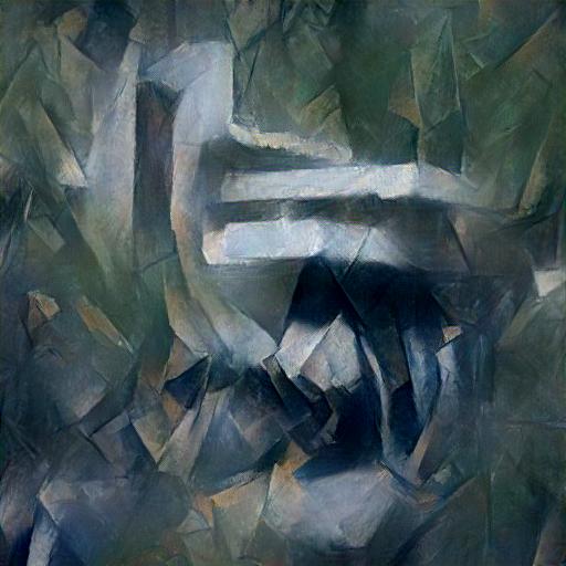
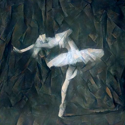
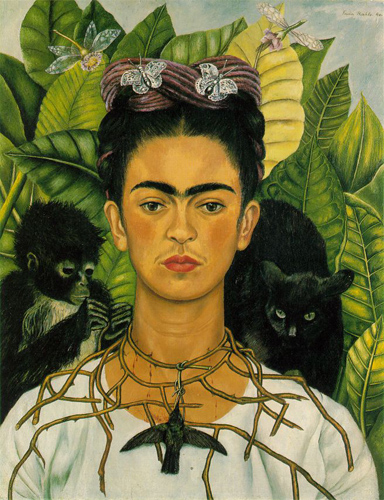
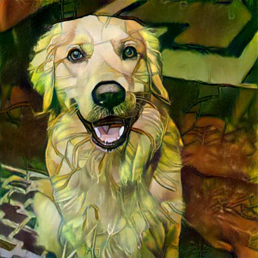
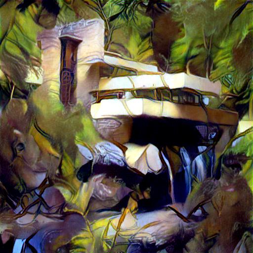
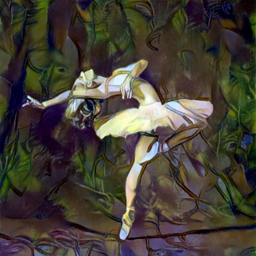
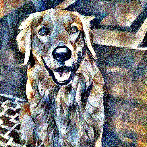
In the above experiments, we take the content image as the starting point of the input image to perform stylization. Here we try to start with random gaussian noise. The optimization process is more sensitive to the balance between the content loss and style loss so that we need to manually find a good set of weights: $\lambda_{\text{style}}=10^6$ and $\lambda_{\text{content}}=10^3$. However, for starting from noise, even though I set 3x number of steps, and it thus take 3x time to process, the result is still worse than starting from content image. Here are the results:

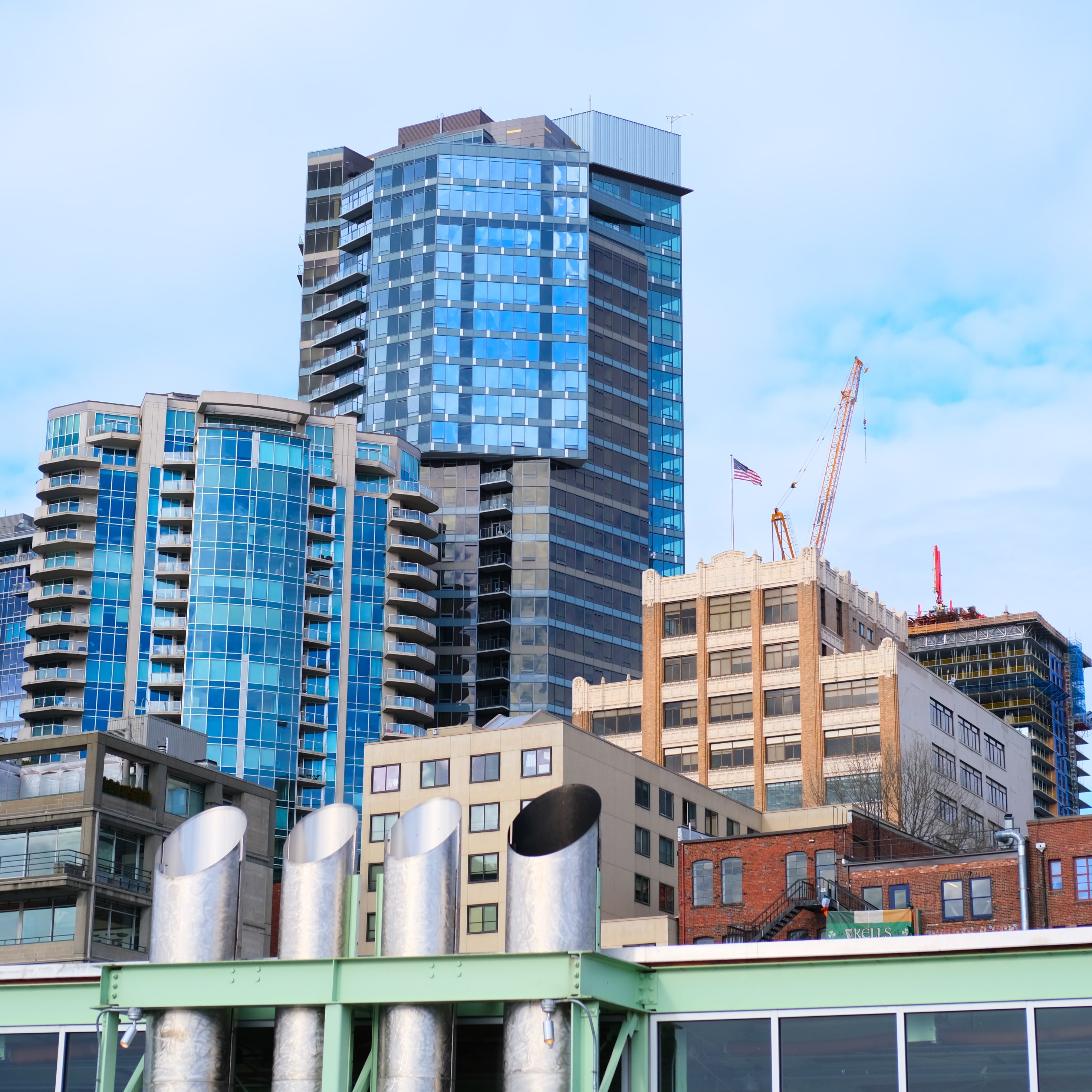
Now it's time to transfer my own picture taken in Seattle into another style:


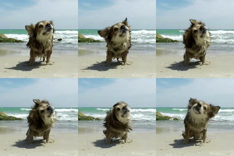
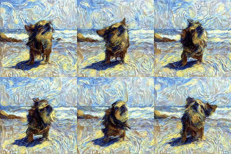
Extra: Stylize a Video!
Here we stylize a video in a frame-by-frame manner.

Extra: Feed Forward Network
Rather than directly optimizing the input picture, we can optimize a feedforward network to perform image stylization. Here we use the generator of CycleGAN from project3 as the feedforward network to stylize the fallingwater image into the texture of stary-night style. The feedforwrd training process is very sensitive to the hyperparameters. Here are the results with different hyperparameters:
