Toy Problem
Gradient Constraint & Value Constraint
Image gradient describes the change in pixel intensity, and together with the value of one pixel, we can reconstruct the original image. I consider these two types of constraints as gradient constraint and value constraint. The gradient constraint describes the shape of the image (i.e., the gradient), and the value constraint describes the color of the image (i.e., the pixel intensity in each channel).
Both gradient and value constraints are necessary to reconstruct the original image. The value constraint acts as an anchor to prevent the values from floating around. In techniques like Poisson blending and mixed gradient blending, the distinct roles of these two constraints become apparent: the gradient transfers the shape, and the value matches the color.

2 Types of Constraints
Constructing Linear Equations
The image reconstruction problem can be formulated as follows: $$ \text{argmin}_v \left[\text{Dist}(\text{grad}_x(v), \text{grad}_x(s)) + \text{Dist}(\text{grad}_y(v), \text{grad}_y(s)) + \text{Dist}(\text{value}_{(0,0)})\right] $$ where $\text{Dist}$ is the distance function, $\text{grad}_x(p) = p(x+1,y)-p(x,y)$ and $\text{grad}_y(p) = p(x,y+1)-p(x,y)$ represent the gradient of image $p$ in the x and y directions, respectively, and $\text{value}_{(0,0)}$ is the value of the pixel at (0,0). This optimization problem can be reformulated into an equivalent linear equation $A \cdot v = b$ and solved using the least squares method.
Specifically, I prefer to construct the matrix $A$ and vector $b$ one direction at a time, i.e., in the order of $\text{Dist}(\text{grad}_x)$, $\text{Dist}(\text{grad}_y)$, $\text{Dist}(\text{value}_{(0,0)})$. I chose the csr_matrix, as recommended by ChatGPT, for efficient matrix multiplications. The final linear equation $A \cdot v = b$ is then solved using scipy.sparse.linalg.lsqr().
An important detail is that since the gradient is symmetric between neighboring pixels, it is only necessary to consider the gradient between the right and bottom pixels.
A Pixel and her neighbors
Gradient in two directions
The reconstructed image is displayed below. Additionally, I conducted experiments by removing the value constraint, which revealed that the pixel intensity shifts randomly due to the absence of a base value.

Toy Problem Result

Toy Problem without Value Constraint
Poisson Image Editing
Similar to the toy problem, the Poisson image can be formulated as follows: $$ \text{argmin}_v \left[\sum_{\Omega}\text{Dist}(G(v,s)) + \sum_{\partial\Omega}\text{Dist}(V(v,t,s))\right] $$ where the first part $\sum_{\Omega}\text{Dist}(G(v,s))$ represents all the gradient constraints within the masked area $\Omega$, and the second part $\sum_{\partial\Omega}\text{Dist}(V(v,t,s))$ represents the value constraints on the boundary $\partial\Omega$. More specifically: $$ \text{Gradient Constraints: } \sum_{\Omega}\text{Dist}(G(v,s)) = \sum_{i \in \Omega,\ j \in N_i \cap \Omega}\left(v_i-v_j - (s_i-s_j)\right)^2 $$ $$ \text{Value Constraints: } \sum_{\partial\Omega}\text{Dist}(V(v,t,s)) = \sum_{i \in \Omega,\ j \in N_i \cap \partial\Omega}\left(v_i-t_j - (s_i-s_j)\right)^2 $$ Here, $i$ is every pixel in the masked area $\Omega$, $j$ are the neighbors of $i$ $(j \in N_i)$, $v$ are the pixels we want to solve, $s$ is the source image (foreground), and $t$ is the target image (background).
Intuitively, we want the resulting image $v$ to retain the texture (gradient) of the source image $s$ (foreground) but also blend seamlessly into the color space of the target image $t$ (background).
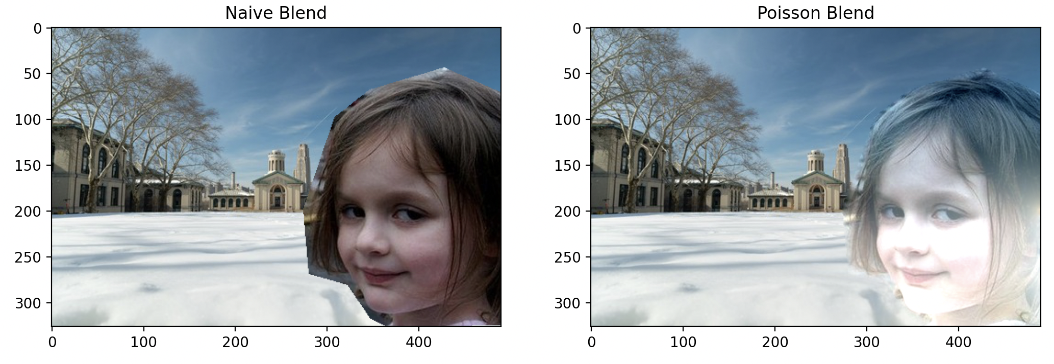
The girl from the meme came to CMU!
As we can observe, the algorithm managed to blend the edges decently. However, the snow and sky's coloration causes her face to appear slightly overexposed, and she has blue hair now.
Let's try a different background.
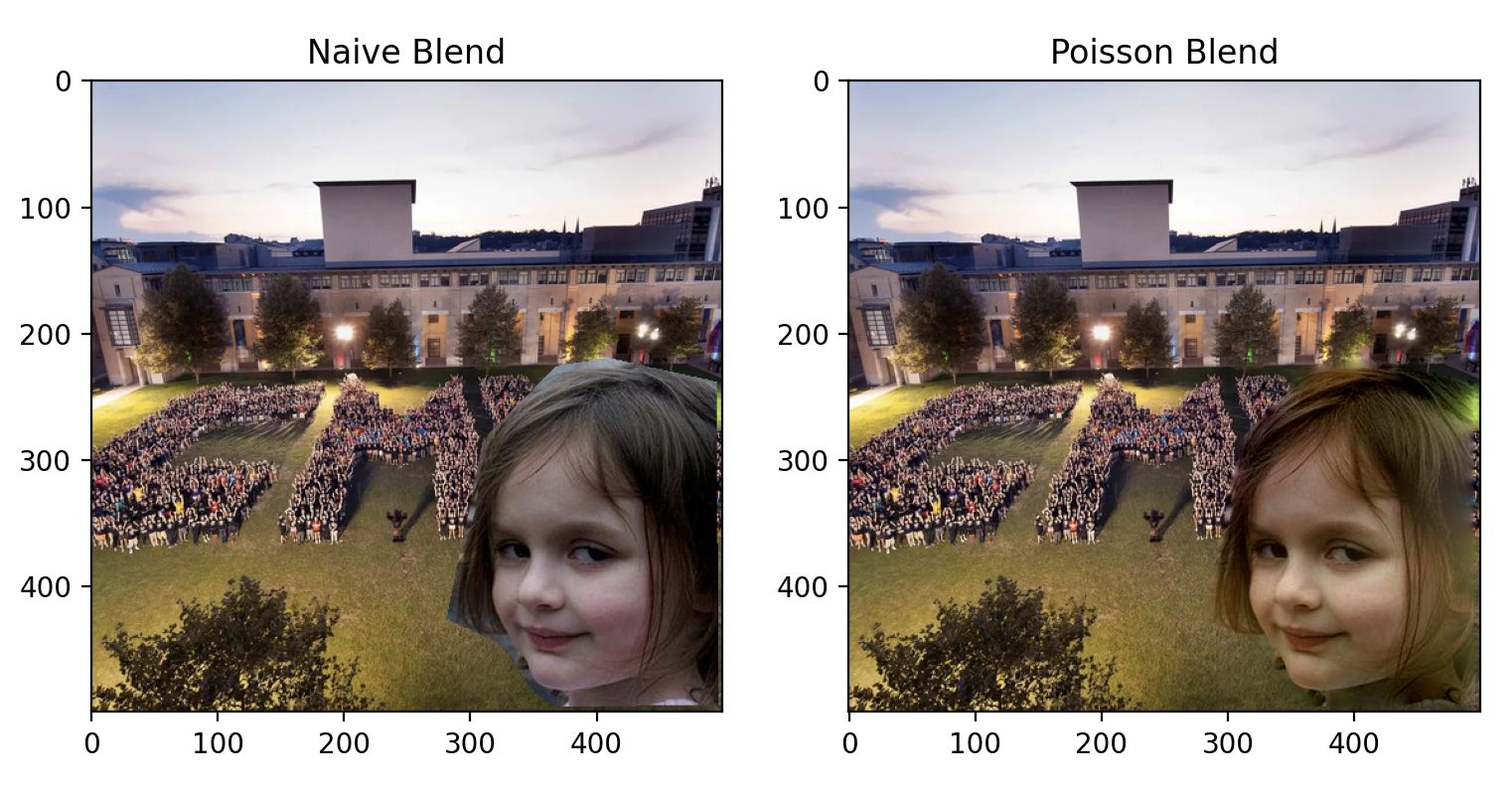
She wants a selfie with the students.
The lighting in this image is more favorable. But, the green hue of the grass still bleeds into her face. Let's try adding a black border to the image.
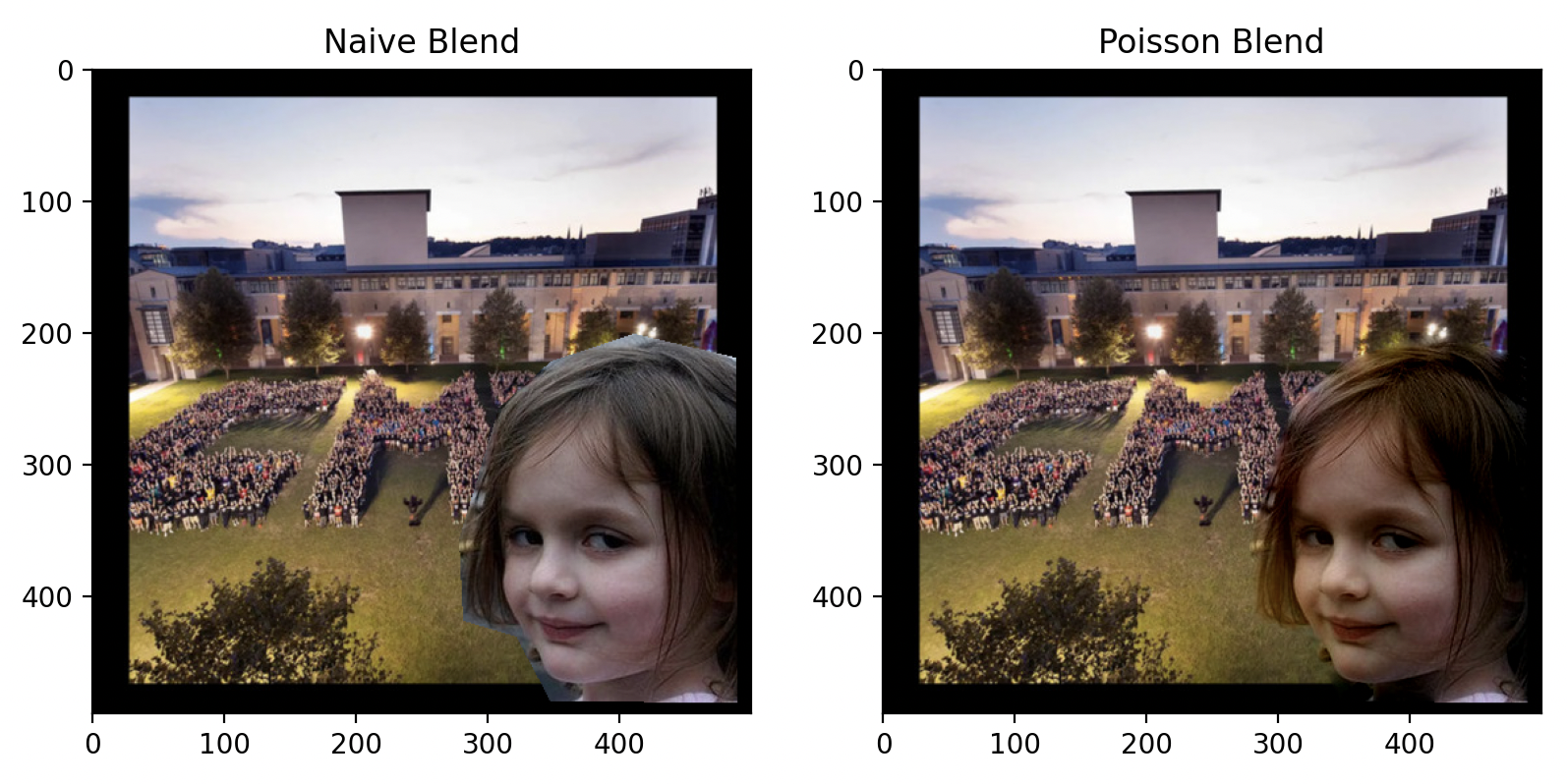
She is satisfied.
Now the image is perfect! The lighting is slightly warm, matching the background beautifully. Notice how Poisson blending impeccably aligns the details of her hair with the grass.
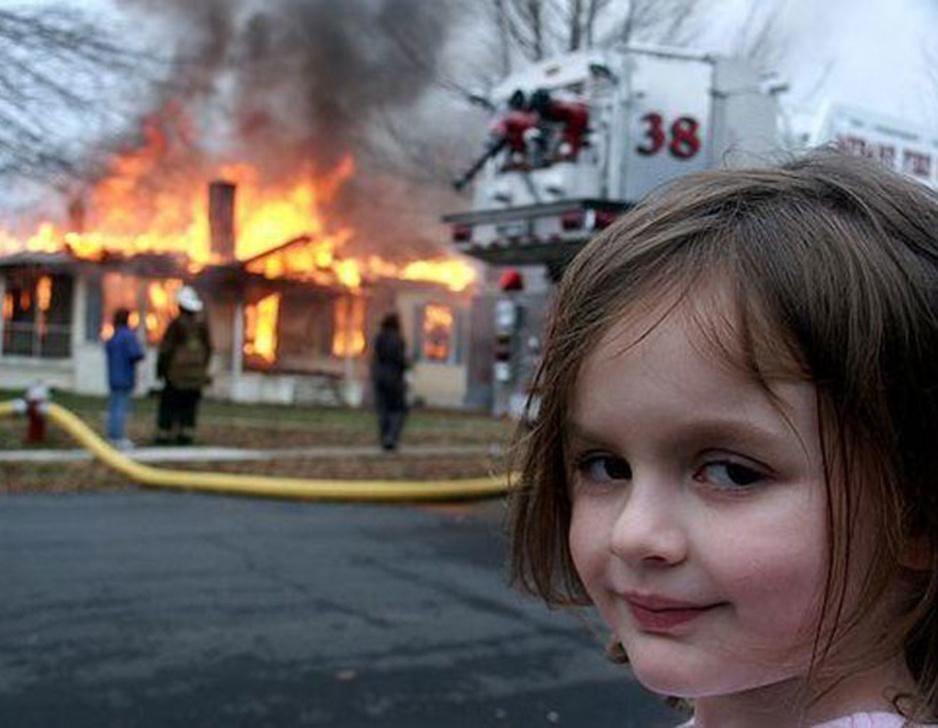
Original Meme
We can conclude that in order to get the ebst results, the forground needs a border as "padding" to prevent the color of the background from bleeding into the object. And possion works best with clean object with no holes, the background near the object should also be as clean as possible.
Failed Examples
Poisson blending utilizes only the foreground gradient as a guidance field, which can sometimes lead to undesired results. The following image demonstrates a failed example of Poisson blending, where the color bleeds into the object and unnecessary texture at the border is preserved.
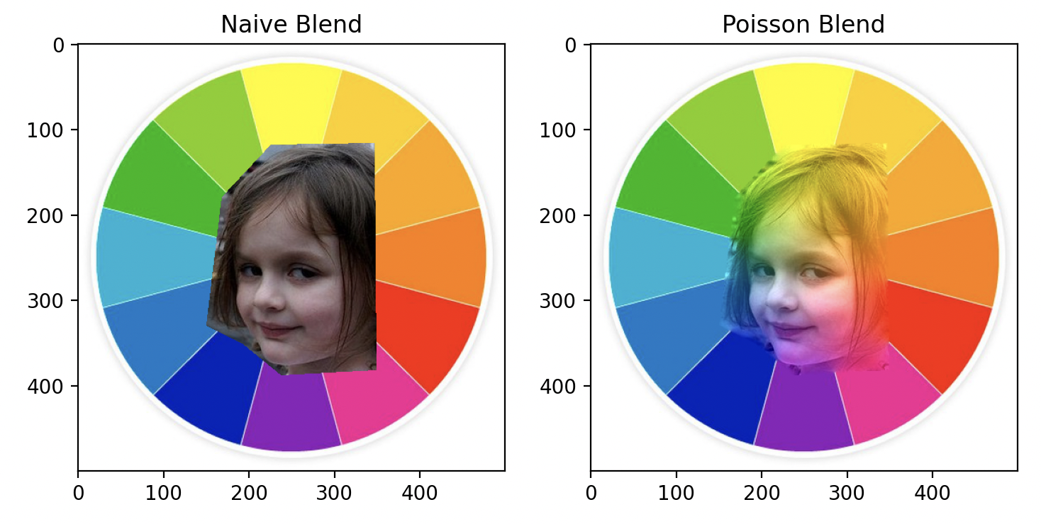
Girl and Color Wheel
Poisson blending also struggles to handle objects with holes and non-convex shapes. Observe the area near the boy's arm and leg for an example of this limitation.
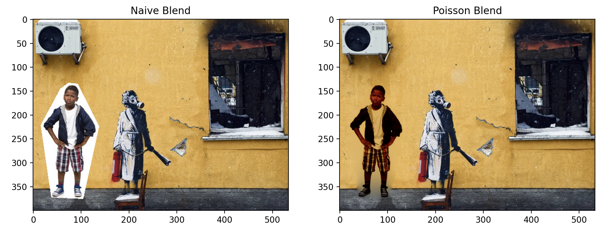
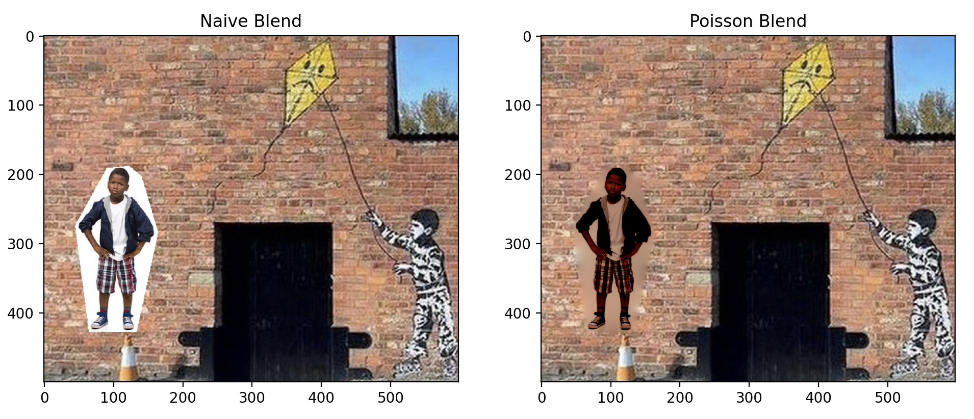
Banksy and Boy
Improvements
Mixed Gradient
Instead of solely utilizing the gradient from the foreground, we can enhance the guidance field by incorporating the gradient from the background as well. This is achieved by retaining the larger value of each gradient, effectively "mixing" the textures from both the foreground and the background. This approach is particularly advantageous when dealing with transparent objects or painting.
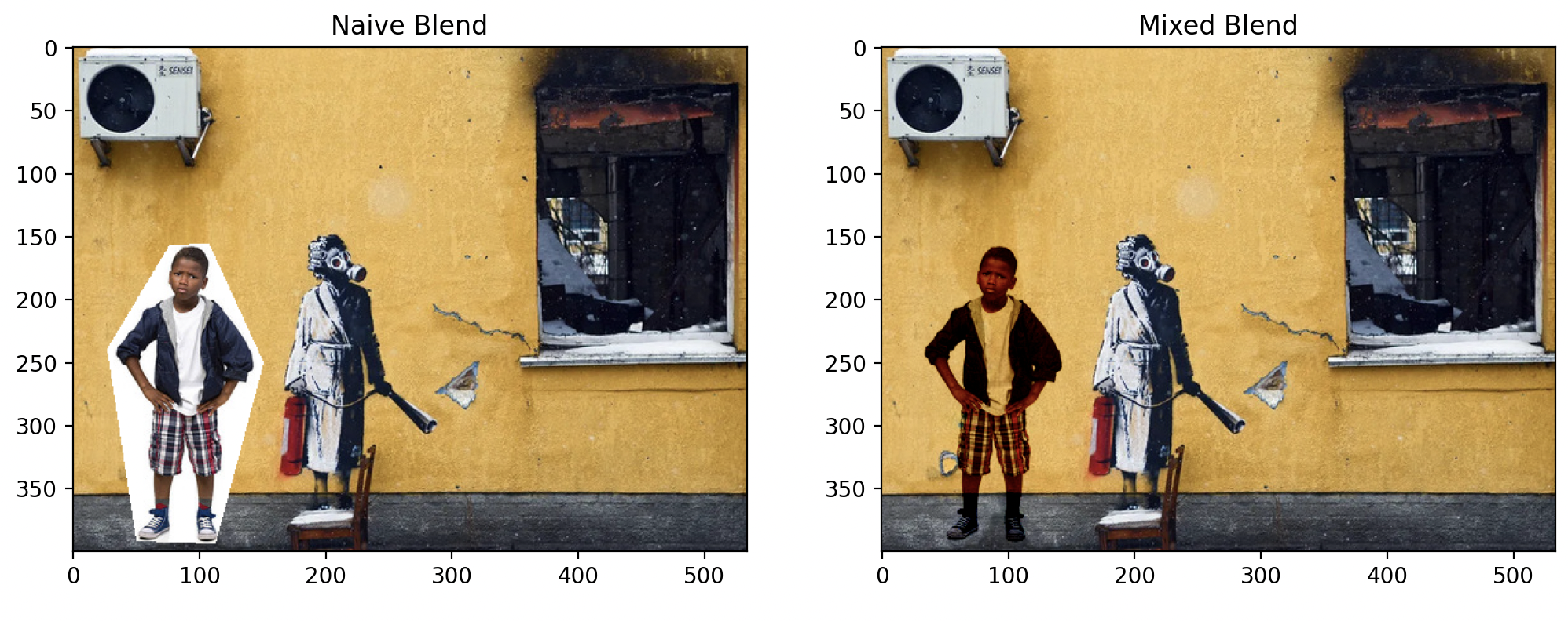
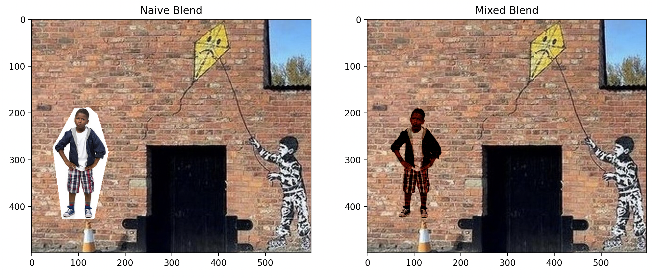
Notice the improvement near the arm and legs.
Highlighting Objects
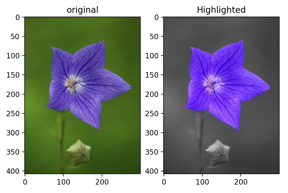
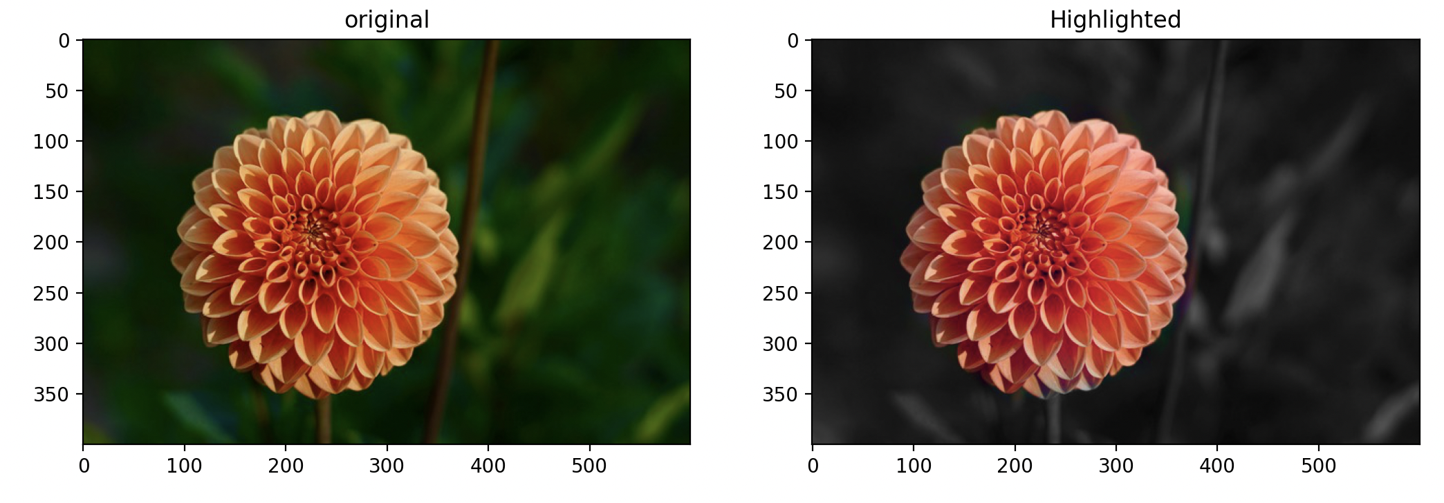
Just as modifying the gradient constraint with mixed gradients alters the blending outcome, adjusting the value constraint can also produce varied effects. By designating the background's luminance from the original image, we can "force" the background to appear gray, effectively highlighting only the target object. The result is surprisingly effective, as demonstrated below.
Highlighted Flowers
Color2Gray
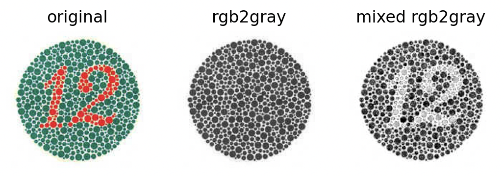
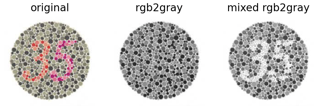
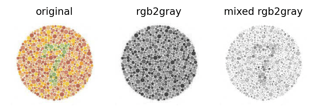
As part of the additional features, I implemented an improved version of the color2gray algorithm, which is capable of preserving the color patterns in images. This enhancement is achieved by extracting the gradient field in the Saturation and Value channels of images. As demonstrated below, these two channels effectively represent the color patterns.
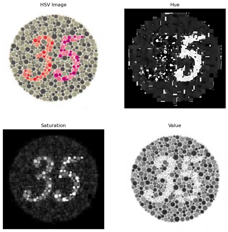
Visualizations of HSV Channels Separately
By combining the gradient fields, we can approach this as a mixed gradient blending problem. The outcome is illustrated below. One important detail is that since the mask generated for the image is not perfect, we need to invert the pixel values in the Saturation channel to prevent the color bleeding problem.

Color Constancy
Do you still remember this dress? What color do you think it is?
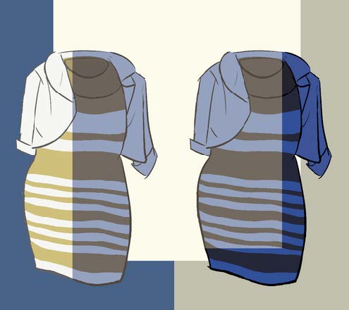
Maybe you already know the two squares are the same color in the following image. But do you feel the same?
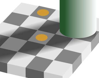
Our visual system uses a variety of tricks to make sure things look the same color, regardless of the illuminant (light source). This phenomenon is known as color constancy. Take a look at the following image.
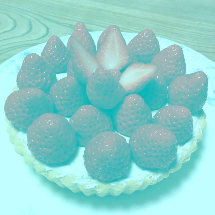
What color do you think the strawberries are?
In reality, all the pixels in this image are shades of blue and gray. Surprising, isn't it? We can examine the pixel color distribution to confirm:
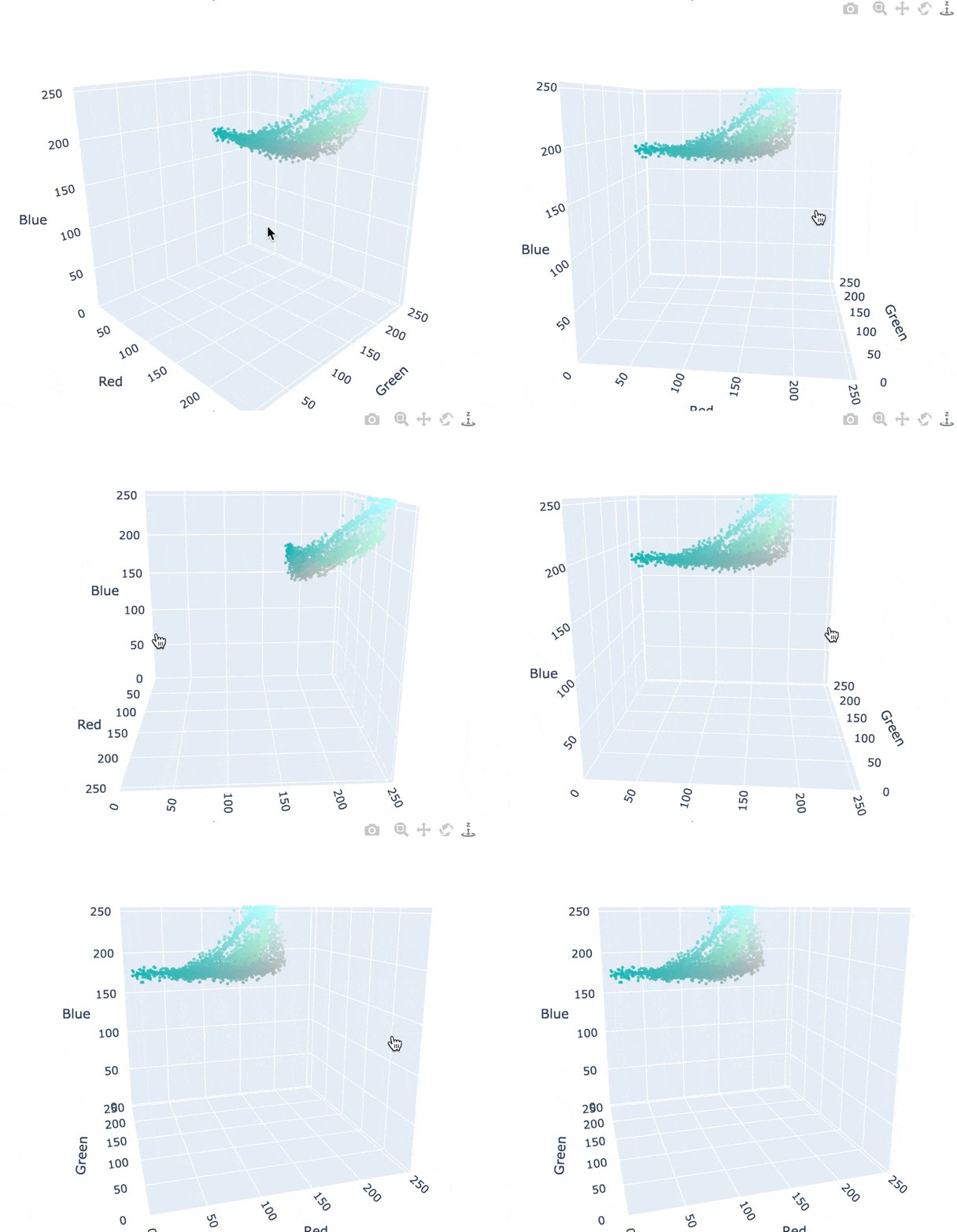
Vice published a great article on this subject. Here's a key excerpt:
"In this picture, someone has very cleverly manipulated the image so that the objects you're looking at are reflecting what would otherwise be achromatic or grayscale, but the light source that your brain interprets to be on the scene has got this blueish component," Conway(some expert) told me. "You brain says, 'the light source that I'm viewing these strawberries under has some blue component to it, so I'm going to subtract that automatically from every pixel.' And when you take grey pixels and subtract out this blue bias, you end up with red."
With Poisson blending, we can create images that similarly play tricks on perception. For instance, I crafted this banana to look yellow, although most pixels are actually bluish gray.
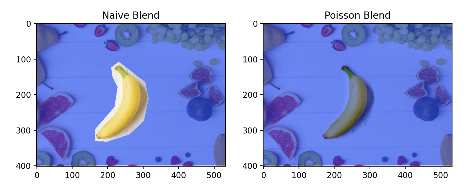
This requires additional fine-tuning; some pixels still appear grayish-yellow.
Image Reillumination
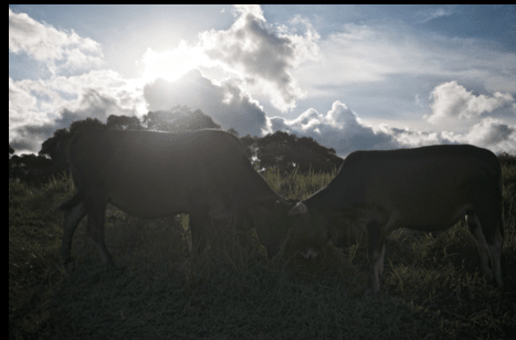
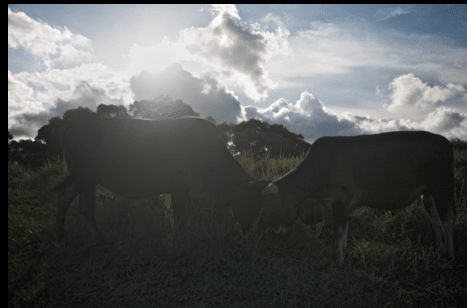
The original paper demonstrated the use of Poisson image editing to smooth the gradients of an image, thereby adjusting overexposed and underexposed areas. This technique was proposed in this paper. Generally, we can apply this technique by adjusting the guidance gradient field as follows: $$ \mathbf{v}=\left(\frac{0.2\left\langle\nabla f^*\right\rangle}{\left|\nabla f^*\right|}\right)^{0.2} \nabla f^* $$ where $\left|\nabla f^*\right|$ is the average gradient of the target area, and $f^*$ represents the target image.
I applied this technique to restore details of the cloud near the sun. The result is shown below.
Compare the original and reilluminated images.