Project 4 - Style Transfer
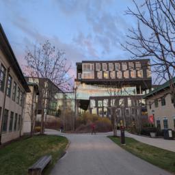
Boring Gates Hall
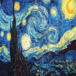
Style Target
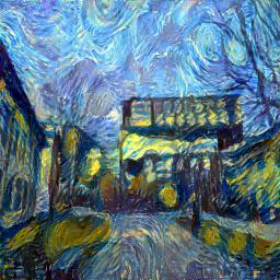
Stytlized Gates Hall
Sometimes, real life becomes very boring, with the same thing over and over again in a never-ending cycle. In contrast to real life, art is creative, imaginative, and varied. What if we can bring art into real life? Enter style transfer. Style tranfer aims to blend the style of one image into the contents of another by optimizing for both content loss and style loss. Content loss is calculated via the l2 of set intermediate layers in a pretrained network and the style loss is calculated via the distance between gram matricies of intermediate layers. Optimizing style and content loss together can create some beautiful images.
Content Reconstruction
We implement content reconstruction by selecting layers from VGG19 as loss layers. For each loss layer, we compute the layer difference between input and target image and minimize that error. We compare the differences of minimizing different layers of the VGG19 pretrained network.
Figure. Content reconstruction at different layers.
- We see that using features from conv_1 almost perfectly reconstructs the image. This makes sense because conv_1 has not been pooled and contain a lot of information from convolutional kernels for each pixel.
- We see that conv_2 reconstructs the image well, but loses color accuracy.
- We see that conv_3 retains the edges and shapes of the image but loses the correct texture and colors. This makes sense because the later convolutional layers are running on pooled features and encodes larger, higher level features.
- For conv_4 we are barely able to make out the dog in the image.
- For conv_5 it is very very hard to see the dog. This because conv_5 features are very abstract and contain more information on classes used to train ImageNet rather than information about the image itself.
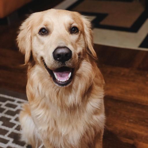
Target Content Image
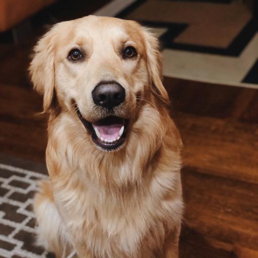
conv_1 reconstruction
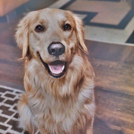
conv_2 reconstruction
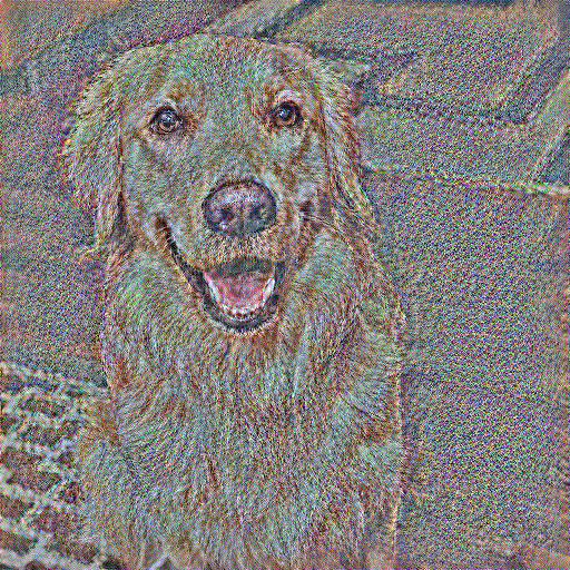
conv_3 reconstruction
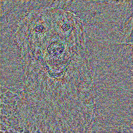
conv_4 reconstruction
conv_5 reconstruction
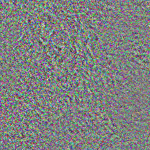
Figure. Random Noise Reconstruction on conv_1. My favorite layer for reconstruction is conv_1 because the reconstructed images look really realistic.
While conv_1 is good at reconstruction in isolation, it is not ideal for style transfer because it enforces too much low level textures and colors that we want to import from the style image instead.
Since conv_1 nearly perfectly reconstructs the image from random noise, we don't see a visible difference between images reconstructed from different random noise.

Content Input

Random Init 1

Random Init 2
Texture Synthesis
Now we perform texture synthesis. Since for texture we do not care about pixel-wise correspondence but rather the overall pattern, we minimize the distance between the gram matricies of input and target image at set intermediate levels. We notice that earlier levels encode color and fine texture while later levels encode larger texture patterns with the higher field of view.
Figure. Texture Synthesis with Varies layers
- We see that generally earlier conv layers encodes color and local texture and edges while later layers encodes higher level information.
- Texture with conv1+2+3 is very vibrant and expresses lots of accurate color and edges, but it lacks larger swirls and brush lines.
- Texture with conv3+4+5 lacks accurate color and edges. We see that earlier conv layers are very crucial to texture synthesis.
- Texture with conv1+2+3+4+5 encodes a good middle ground of color, edges, and larger brush strokes and swirls.
- Texture with conv2+3+4+5 lacks the vibrant colors and does not look good.
- Texture with conv1+2+3+4 is my favorite with a good representation of colors and edges and also some larger brush strokes.
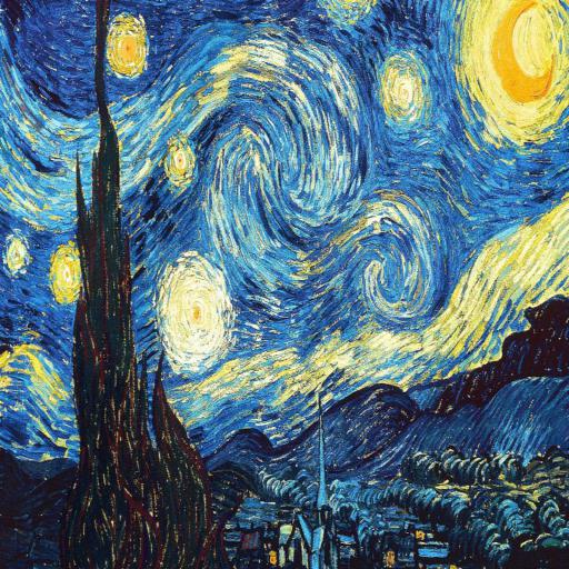
Texture Target
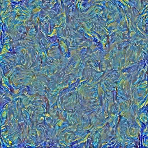
Texture Synthesis conv1+2+3+4
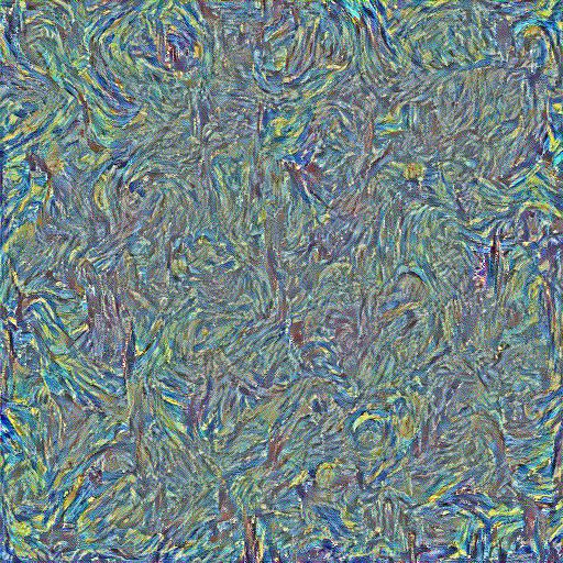
Texture Synthesis conv2+3+4+5
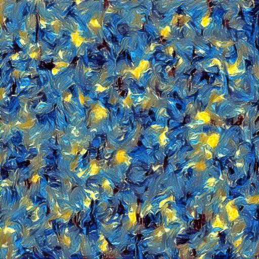
Texture Synthesis conv1+2+3
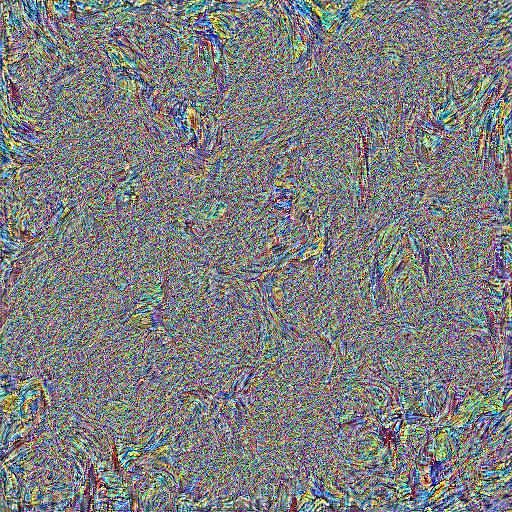
Texture Synthesis conv3+4+5
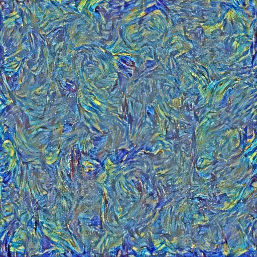
Texture Synthesis conv1+2+3+4+5
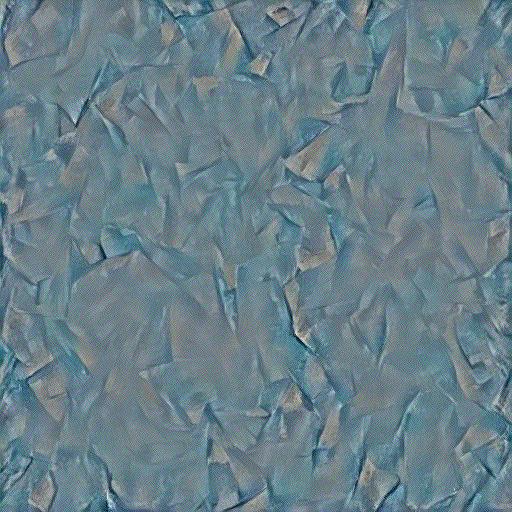
Figure. Random noise texture synthesis. We use conv1+2+3+4 to synthesis picasso texture.
We see that both synthesized textures capture the color and edges of picasso decently well. Although portions of larger areas of darkness and shadows are not included.
We see that the two random initialized outputs both converge to a very similar texture, color, and edges. At the same time, the location of the edges and features are slightly different.
This is due to the different random initialization. We see that random initialization can generate textures very well.

Texture Target
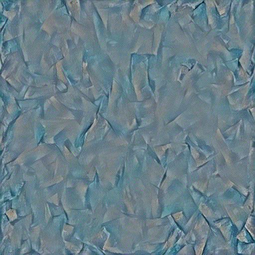
Random Init 1
Random Init 2
Style Transfer
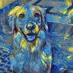
For style transfer, we simply optimize both content loss and style loss at the same time. For style loss, we normalize the gram matricies by dividing by C*H*W, the channel, height, and width, of a specific feature layer. Tuning the hyperparameters of content and stlye loss is extremely and various with the end result you want to get. If you want a stylized image that is a slight modification of the content image, then we need relatively lower style loss weight compared to the style loss weight used to create more expressive results. In general, when initializing from random, we use a style loss weight of 1,000 and content loss weight of 1. When initializing from content image itself, we have a style loss of 1e8 and content loss of 1e-1. This drastic difference is beacuse we only train for 30 steps with the lbfgs optimizer with learning rate 1. Training for 300 steps on my hardware takes 30+ minutes and is computationally prohibitive. Therefore, my hyperparameters may be more aggressive to get to a desired results in shorter iterations and may look different when the training converges. For all results, we optimize conv_2 and conv_3 for content loss and optimize conv_1, conv_2, conv_3, and conv_4 for style loss. We notice that picking conv_1 for content loss is too restricting.
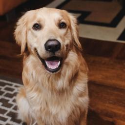
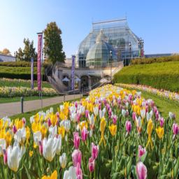
Figure. Grid from random noise. We initialize from random noise and optimize style and content with hyperparameters given above. We optimize for 30 steps with lbfgs. The running time is about 1-3 minutes depending on resolution. We notice that generally, style dominates when optimizing for a short time. Thus, I decreate the weight of style loss to make desirable outputs with just 30 steps.
Source Content Wally
Source Content Phipps

Style Target Starry
Noise Initialize Output
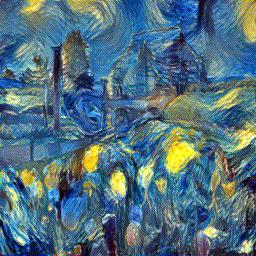
Noise Initialize Output
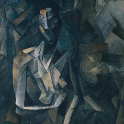
Style Target Picasso
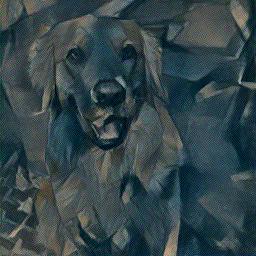
Noise Initialize Output
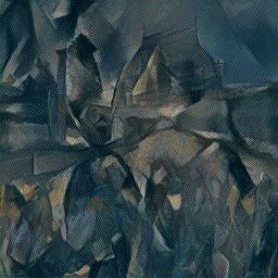
Noise Initialize Output
Figure. Grid from content image. Initializing from content gives a strong bias to the content image. Thus, we increase the style loss weight to arrive at a desirable output with only 30 steps of optimization. We notice that compared to random initialization, we retrain better colors and more details from the content image while the random initialization has more expressive texture. We especially notice a difference for the phipps images where initializing from random ignores a lot of the high frequency details of the flowers given our choice of conv2 and conv3 for content loss. Meanwhile, initializing from content image itself creates an output that better expresses high frequency details at 30 steps. Personally, I like output from content initialization better. The running time is roughly the same given that I use the same 30 steps. I had to increase style loss to get better style at just 30 steps.

Source Content Wally

Source Content Phipps

Style Target Starry
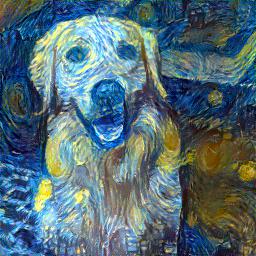
Content Initialize Output
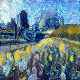
Content Initialize Output

Style Target Picasso
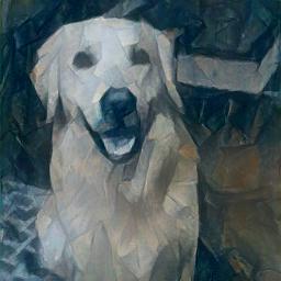
Content Initialize Output
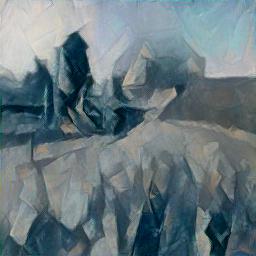
Content Initialize Output
Figure. Using some of my favorite images and Content Initialization.

Source Content Gates
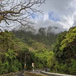
Source Content Hawaii

Style Target Starry

Content Initialize Output
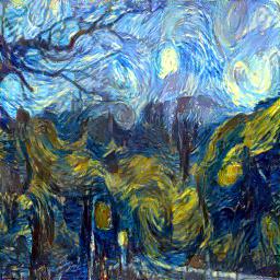
Content Initialize Output
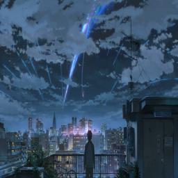
Style Target Your Name

Content Initialize Output
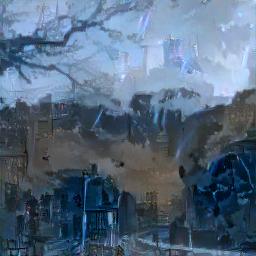
Content Initialize Output